Deep Neural Network
Introduction
Despite the fundamental ideas behind deep learning have been around since 1940s, only recently performance boosted. This rapid progress is due to a combination of complementary factors:
- Large Labeled Datasets that enable models to learn more complex and generalizable patterns.
- Computational power
- Training on GPUs
THE CHALLENGE OF DATA REPRESENTATION
In traditional machine learning algorithms, the performance of a model depends heavily on manually designed features created by human experts. These handcrafted features capture only limited aspects of the data, so once they are fixed, model performance eventually stops improving.
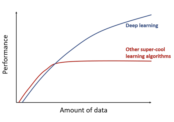
In contrast, deep learning automatically learns useful representations directly from data, building increasingly complex and abstract features as more data becomes available. This ability to learn its own features allows the model to continue to improve by learning increasingly rich and abstract representations.
Linear Classifiers
We consider a Linear Classifier a linear function that maps a -dimensional input space into a -dimensional output space, where corresponds to the number of classes.
So let’s assume we have a training dataset of images
that we want to classify into distinct classes. Thus, the training set is made by couples:
Our goal is to define a function:
that maps images to class scores.
EXAMPLE
Consider the CIFAR-10 dataset, which contains images of size with three color channels , belonging to 10 distinct classes.
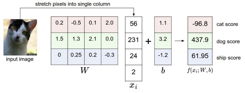
Each image can be represented as a column vector:
We define a linear mapping as follows:
where the parameters are:
- Weight matrix: , containing one row of weights for each class (10 rows in total, each with 3072 elements).
- Bias vector: , which allows the model to shift the outputs so that each class can be centered around zero. This is useful because the input data may not be naturally centered with respect to the origin.
When a new input image is provided, the model outputs a vector of scores, one for each of the 10 classes. The predicted class is the one corresponding to the highest score.
Goal: Learn the parameters and from the training data so that, for any new test image, the score of the correct class is higher than the scores of all other classes.
However, these raw scores are often difficult to interpret directly. To obtain probabilistic predictions, we apply a logistic (or softmax) function, which maps the scores to values between 0 and 1, representing the estimated probability of each class.
LOGISTIC REGRESSION
The logistic regression model is primarily used for binary classification, that is, when we have only two possible classes (e.g. cat vs. not cat).
If we add a sigmoid nonlinearity to our linear mapping, we get a logistic regression classifier:
This model is trained by minimizing the binary cross-entropy loss:
where:
- is the number of examples in the training set
- whith an abuse of notation denotes
- represents the true binary label of each example
In this case the label acts as a selector:
- For positive examples → the model is penalized when the predicted probability is close to 0.
- For negative examples → the model is penalized when the prediction is close to 1.
SOFTMAX CLASSIFIER
The Softmax Classifier is a generalization of Logistic Regression to the multi-class classification. In order to map raw class scores into interpretable probabilities, we apply the softmax function, defined as:
Intuitively, for each class we exponentiate its score , then divide it by the sum of the exponentials of all class scores.
So, the softmax function takes a vector of arbitrary real-valued scores and squashes it into a vector of positive values between 0 and 1 that sum to 1.
it’s important to note that the transformation is nonlinear: the largest score is amplified (pushed toward 1), and the others are suppressed (pushed toward 0).
TRAINING SOFTMAX CLASSIFIER
In the Softmax Classifier, the outputs of the linear mapping:
are interpreted as unnormalized log probabilities — often called logits.
To train the classifier, we use the cross-entropy loss, which measures the distance between the true output distribution and the predicted distribution:
where:
- is the ground truth output distribution (typically a one-hot vector indicating the correct class),
- is the predicted output distribution obtained after applying the softmax.
Notice: The softmax classifier has the appealing property of producing an easy-to-interpret output, i.e., the normalized score confidence for each class.
Modelling a Neuron
Neural networks are a mathematical model loosely inspired by the structure and function of the human brain.
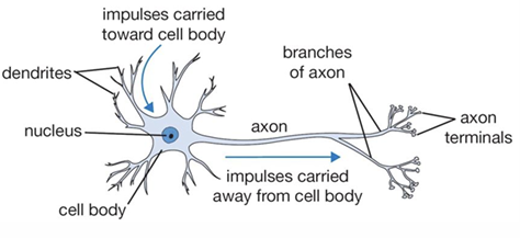
In the brain, neurons are the fundamental computational units. The human nervous system contains approximately 86 billion neurons, interconnected by roughly synapses. Each neuron receives input signals through its dendrites, processes these signals in its cell body (nucleus), where synapses combine the incoming signals into a single output. If the total signal exceeds a certain threshold, the neuron “fires,” sending an output signal along its axon, which branches out to connect with dendrites of other neurons.
Dendrites are embedded in a gel-like substance whose properties influence how strongly incoming signals are amplified or attenuated, affecting the overall behavior of the neuron.
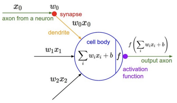
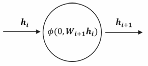
MODELING A SINGLE NEURON
More formally, we can model a single neuron as follows:
-
Inputs and weights
Each neuron receives multiple inputs , which can be amplified or suppressed by corresponding weights .
We can also include a bias term to adjust the threshold for activation.
-
Linear combination
The neuron computes a weighted sum of its inputs:
-
Non-linear activation
The result of the linear combination is then passed through a non-linear activation function to produce the output of the neuron. So, the neuron’s output is the dot product between the inputs and its weights, plus the bias: then, a non-linearity is applied.
A single neuron with a sigmoid activation can naturally implement a binary classifier, and applying gradient descent on its loss is equivalent to optimizing a binary Softmax classifier (i.e., logistic regression).
NEURON ACTIVATION
Activation functions are non-linear functions applied to the output of each neuron. They allow neural networks to approximate complex, non-linear mappings. Among the most widely used historically there are:
-
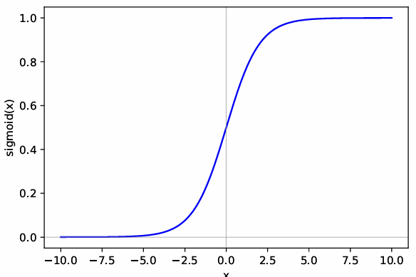
Sigmoid Function
The sigmoid function is defined as:
It squashes any real-valued input into the range . While it was widely used in the past, it is now rarely preferred due to two major drawbacks:
-
Saturates and kills the gradient
- For large positive inputs (e.g., ) the output approaches 1.
- For large negative inputs (e.g., ) the output approaches 0.
In these saturated regions, the derivative of the sigmoid is almost zero, so gradient descent provides very small or no update, slowing learning.
Practically, the model might output 1 for very different scores (e.g., 5 or 600), because the gradient does not distinguish them, so the network cannot adjust efficiently.
-
Not zero-centered
When the input is 0, this means that even with zero input, the neuron outputs a non-zero value, which can introduce unwanted bias during learning and slow convergence.
-
-
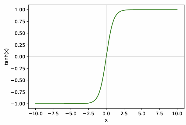
Tanh
The tanh function can be seen as a scaled version of the sigmoid:
Unlike the sigmoid, which maps inputs to , tanh squashes inputs to the range . This makes the output zero-centered, solving one of the main limitations of the sigmoid: when the input is 0, the output is also 0, reducing bias in gradient updates and helping optimization. However, tanh still suffers from saturation for large positive or negative inputs.
-
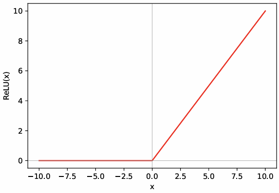
Relu
ReLU stands for Rectified Linear Unit and is defined as:
This activation function is widely used in modern neural networks because it greatly accelerates the convergence of stochastic gradient descent (SGD) compared to sigmoid or tanh functions.
The behavior of ReLU is simple:
- For negative inputs, it outputs 0.
- For positive inputs, it outputs the input itself.
ReLU is non-linear because the operation is not a linear function — it introduces a “kink” at zero, breaking linearity.
Why Non-Linear Activations Are Necessary?
The key reason to use non-linear activation functions in neural networks is that the composition of linear functions is itself linear. Without non-linearities, a neural network, no matter how many layers it has, would effectively reduce to a single-layer linear model, such as logistic regression.
For example, consider a two-layer network with non-linear activations :
If we remove the non-linearities, the function becomes:
This is just a linear transformation, regardless of the number of layers.
Neural Networks
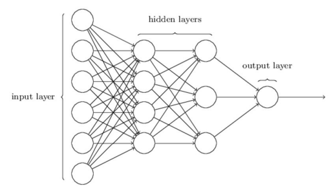
When we connect multiple neurons in layers, we create a Multilayer Perceptron (MLP), the simplest type of neural network.
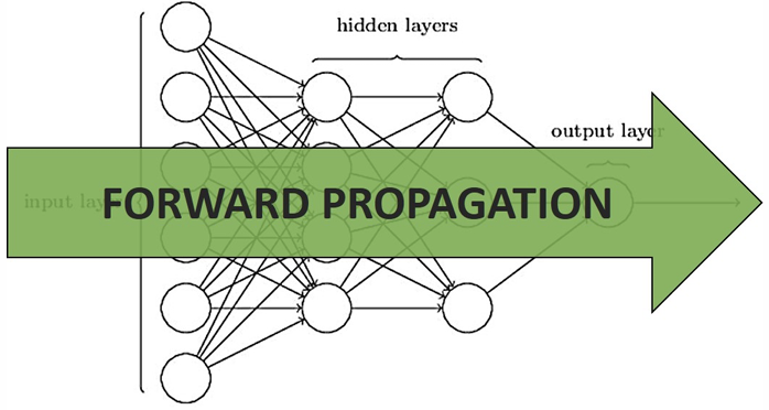
Neural networks are organized in layers:
- Input layer receives the raw input features.
- Hidden layers (N layers) perform intermediate computations using non-linear activations.
- Output layer produces the final predictions.
The key idea is that the composition of non-linear functions performed by the layers allows the network to model complex, non-linear mappings from inputs to outputs.
Some of the characteristics of MLP are:
- Connections: Each neuron in a layer is typically connected to all neurons in the next layer (fully connected).
- Number of neurons: The number of neurons in the output layer corresponds to the number of scores or classes you want to predict. For example, for a 3-class classification problem, the output layer has 3 neurons.
- Independence from input/output size: The structure of hidden layers does not directly depend on the size of the input or output; it depends on the desired expressive power of the network.
EXAMPLE
The previously depicted 4-layer neural network can be expressed compactly as:
where:
- is the activation function,
- is the input vector,
- are the weights of the first layer,
- are the weights of the second layer,
- are the weights of the third layer.
Note: For simplicity, biases have been incorporated into the weight matrices in this notation
FORWARD PROPAGATION
Forward propagation is the process of computing the network output given its input. In other words, it is the step where we perform inference by passing the input through the network.
The formula of forward propagation is the one seen in the previous paragraph.
REPRESENTATIONAL POWER
It has been mathematically proven that any continuous function can be approximated to arbitrary precision by a neural network with at least one hidden layer:
Because of this property, neural networks with at least one hidden layer are called universal approximators.
Why is this important?
By composing functions (i.e., stacking layers), a neural network can approximate even highly complex functions with arbitrarily small error. In practice, this means that if there exists a function that can solve a problem, a sufficiently large neural network can learn an approximation of it.
On a computer, numerical precision is finite, so the theoretical guarantees are approximated in practice.
Adding more hidden layers often improves performance, even if in theory a 2-layer network can represent the same function. More layers help in efficiently learning complex representations and in better utilizing computational resources.
SETTING HYPERPARAMETERS
The number of layers in a neural network, along with the number of neurons in each layer, are known as hyperparameters of the network architecture:
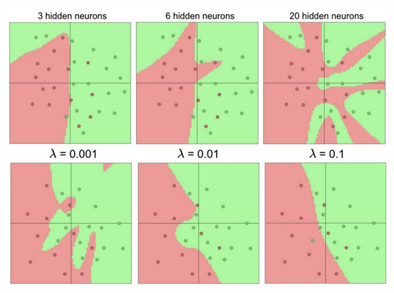
- Increasing the number of layers or neurons increases the capacity of the network, which is good because it allows to capture more complex patterns in the data.
- However, larger networks without proper regularization are more likely to overfit the training data, memorizing it rather than learning generalizable patterns.
In practice, choosing hyperparameters involves balancing network capacity with regularization and available data, to achieve good generalization on unseen examples
Training DNN
In training Deep Neural Networks (DNNs), the objective or loss function measures the quality of the mapping from input to output. This function has a form of this kind:
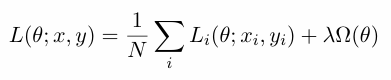
Where:
- is the number of training examples,
- is the set of network parameters
- weights the regularization’s strength.
In particular it is typically composed of two parts:
- The data term, computed as an average over all training examples, evaluates how well the model’s predictions match the true labels.
- The regularization term which depends only on network parameters and has the role to mitigate the risk of overfitting. Since deep models usually have a large number of parameters, we aim to use as few parameters as possible while maintaining good performance — this is achieved through regularization.
There are mainly two types of regularization:
-
L1 Norm
The sum of the absolute values of the parameters. Minimizing this term reduces both the classification error and the sum of the absolute parameter values. The derivative of the L1 norm with respect to a parameter is 1 (for non-zero parameters), which encourages many parameters to become exactly zero, promoting sparsity.
-
L2 Norm
which adds the sum of squared parameters. This makes the parameters smaller in value but does not force them to zero, resulting in smoother weight decay rather than sparsity.
While L1 can create discontinuities in its derivative, L2 provides a continuous relaxation, which is often used in practice to obtain a smooth approximation.
LOSS FUNCTION
Depending on the task we want to solve, we can use different kinds of loss functions:
-
Classification
-
Hinge loss:
The hinge loss measures how much a classifier fails to correctly separate the data, heavily penalizing misclassifications and points that lie close to the decision boundary.
The hinge loss is commonly used for classification problems, particularly in Support Vector Machines (SVMs), where it is introduced the concept of a margin.
For each class , we compute :
- If this value is greater than 1, the instance is correctly classified and sufficiently far from the margin →
- Otherwise, the instance is misclassified or too close to the margin, and the loss increases linearly with the distance from the margin.
-
Softmax loss:
The softmax loss, also known as the cross-entropy loss, is commonly used for multi-class classification problems.
Here, represents the exponentiated score of the correct class , while the denominator sums the exponentiated scores of all classes. The logarithm is applied to ensure numerical stability; it does not change the optimal solution since the logarithm is a monotonic function.
-
-
Regression
-
Mean Squared Error (MSE):
When the task involves predicting a continuous value, we typically use the Mean Squared Error (MSE) loss:
It measures the squared difference between the predicted value and the true value .
-
LEARNING THE PARAMETERS
During the training phase, we want to learn the set of network parameters that minimize the objective (loss) function on the training set.
Formally:
The key difference between logistic regression and neural networks lies in the structure of the function we are optimizing:
- In logistic regression, the loss is a single, simple function of the parameters, and we can compute its derivative directly.
- In contrast, in a neural network, the loss is a composition of many nested functions—each layer depends on the previous one.
Therefore, we cannot directly compute the derivative of the loss with respect to the parameters; instead, we must apply the chain rule of derivative, a process known as backpropagation.
BACKPROPAGATION
The backpropagation algorithm efficiently computes all the gradients of the loss function with respect to its parameters by applying the chain rule of calculus through the network’s layers.
For example, if we have and , the final output depends on through both and . To compute how changes with respect to , we must consider both functions together. This is expressed by the chain rule:
Backpropagation proceeds backwards with respect to the flow of computations used to compute the loss itself — hence the name.
If everything is done correctly, simplifying all the terms on the right-hand will give you the same result as the direct derivative on the left-hand side.
Backpropagation is a local process. Neurons are completely unaware of the complete topology of the network in which they are embedded.
Indeed, in order for backpropagation to work, each neuron just need to be able to compute two things:
-
Derivative of its output with respect to its weights:
-
Derivative of its output with respect to its inputs:
BACKPROPAGATION FLOW
During backpropagation, each neuron receives information about how its output affects the final network loss through the gradient:
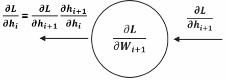
This gradient flows backward from the output layer toward the input layer, allowing each neuron to understand its contribution to the overall error. Once a neuron receives this gradient, it applies the chain rule of calculus to compute the gradient with respect to its own inputs by multiplying the received gradient with its local gradient — the derivative of its activation function. This chained gradient is then passed to the neurons in the previous layer, propagating the error signal backward through the network.
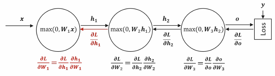
To train the network, we need to update all the weights to reduce this loss. As we said Backpropagation achieves this by sending gradient information backward through the network, starting from the loss and flowing back to each layer.
For the final layer , computing is straightforward because the loss directly depends on the output , which directly depends on . However, for earlier layers like and , the loss doesn’t depend on them directly—there are intermediate layers in between. This is where the chain rule becomes essential.
The Recursive Pattern:
To find we break it into two parts:
- First, how does the loss change with respect to (∂L/∂h₂),
- Second, how does h₂ change with respect to (∂h₂/∂W₂).
The clever part is that itself can be computed by chaining backward from the next layer:
This same pattern continues for . Each layer receives the gradient from the layer ahead, multiplies it by its local gradient (how its output changes with respect to its input), and passes this information backward.
WEIGHT INITILIZATION
When initializing the weights in a neural network, random initialization is crucial to break symmetry and enable effective learning. If all weights were initialized to the same value (e.g. 0), then all neurons in a given layer would compute the same outputs, the same gradient and undergo identical parameter updates.
To avoid this problem, common practice is to initialize weights to small random numbers centered around zero and all biases to zero. These random weights are sometimes scaled according to the neuron’s fan-in (the number of input connections). Scaling is important because a neuron with many inputs could otherwise produce very large outputs even from small weights, potentially leading to numerical instability or saturating activation functions.
Advanced initialization schemes, like Glorot-Bengio (Xavier) initialization, automatically scale weights based on the fan-in (and sometimes fan-out) of each neuron, helping maintain a stable variance of activations across layers. Most modern deep learning frameworks handle weight initialization automatically, offering options such as uniform, Gaussian, or Xavier initialization.
Regularization
Deep networks have very high representational capacity, which allows them to learn very complex functions. However, it also makes larger networks more susceptible to overfitting if not properly regularized during training.
We have already introduced the concept of explicit regularization, which directly incorporates a regularization term into the loss function. In addition to this, there are other neural network regularization techniques that do not require modifying the loss function. These are known as implicit regularization methods, because they help regularize the network during training without explicitly altering the loss function.
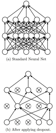
DROPOUT
The first regularization technique which is really peculiar to neural networks is dropout.
The technique works by temporarily “dropping out” neurons with a specified probability at each training step. This means that, at each training step, a neuron can be randomly turned off—its output is set to zero, and it is excluded from both the forward pass and backpropagation.
For example, if a layer has a dropout probability of 0.5, each neuron in that layer has a 50% chance of being active (on) or inactive (off) during a given training step
In effect, dropout samples a different sub-network at each training step, updating only the corresponding subset of parameters. During testing, dropout is not applied. This can be interpreted as computing the average prediction of an ensemble of these sub-networks.
The regularization effect arises because neurons cannot rely on specific neighboring neurons and are prevented from memorizing the training data. This encourages the network to learn more robust and generalizable features.
DATA AUGUMENTATION
One of the most effective ways to improve a machine learning model’s generalization is simply to train it on more data. Overfitting often occurs when the number of model parameters is much larger than the number of available training examples. Unfortunately, collecting additional data is not always possible.
Data augmentation consists of generating new training examples by applying some transformation to inputs in our training set. Of course, is important that these transformations must preserve the original label.
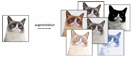
For example, if you have an image labeled “cat,” you can create multiple new images by applying non-destructive transformations such as rotations, flips, or color adjustments. Depending on the number of transformations applied, the effective size of the dataset can increase proportionally
By augmenting the dataset in this way, the model is less likely to memorize the training data, since it must learn to correctly classify different variations of the same input.
EARLY STOPPING
During training, it is common to set aside a small portion of the data as a validation set. A typical sign of overfitting is when the training loss continues to decrease while the validation loss starts increasing. This divergence indicates that the model is beginning to memorize the training data rather than learning to generalize.
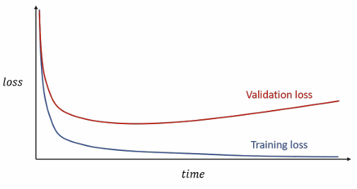
Early stopping addresses this by stopping the training process when the validation loss stops improving. In practice, we often introduce a patience parameter, which defines the number of additional epochs to wait in which the validation loss is stable (or started increasing) before actually stopping the training.
Key Takeaways
| Concept | Formula / Description |
|---|---|
| Linear classifier | |
| Sigmoid | — range , saturates at extremes |
| Tanh | — range , zero-centered |
| ReLU | — no saturation, default choice |
| Softmax | — maps scores to probabilities |
| Cross-entropy loss | |
| MSE loss | |
| Chain rule | — the basis of backpropagation |
| L1 regularization | $\Omega(\theta) = \sum |
| L2 regularization | — smooth weight decay |
| Dropout | Randomly disable neurons with probability during training |
| Data augmentation | Generate new training examples via label-preserving transformations |
| Early stopping | Stop training when validation loss stops improving |