Transformers
Temporal Convolutional Architectures
INTRODUCTION
A sequence model is a model that takes in input a sequence of items (words, letters, time series, audio signals, etc) and produce either a single output or another sequence of outputs.

Each position in the sequence is often called a time step. The item at each time step, also referred to as a token, is represented by a set of numerical features.
While sequence modeling is historically associated with Recurrent Neural Networks (RNNs), other architectures such as Convolutional Neural Networks (CNNs) can also be utilized.
CNN
Even though Convolutional Neural Networks (CNNs) are primarily associated with image analysis, their operations can also be effectively adapted for sequence data.
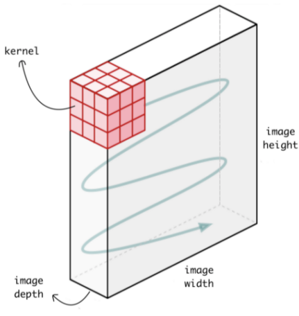
In image processing, a Conv2D operation uses a two-dimensional kernel that slides across the image’s spatial dimensions (height and width). In contrast, for time series or sequential data, this same principle is applied through a Conv1D operation.
In this approach, the kernel is a one-dimensional filter that moves along the temporal axis. This allows the model to preserve critical sequential information, such as:
- Temporal dependencies in time series (e.g., causal patterns)
- Syntactic order in text (e.g., noun–verb–object).
FROM 2D TO 1D CONVOLUTION
When shifting from 2D to 1D, we still operate on multi-featured data. For example, a sentence is a sequence where each token is described by multiple features.
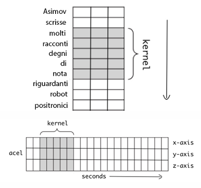
In this context, the 1D convolution kernel (e.g., of size 5) slides along only one dimension: the temporal axis (the sequence length).
There is, however, an “implicit” second dimension: the feature size. The kernel’s second dimension must always match the number of features in the input sequence. For instance, if the input tokens have 3 features and the kernel size is 5, the kernel’s actual shape is (5, 3). It slides temporally, but at each step, it processes all 3 features simultaneously.
The discrete 1D convolution is mathematically defined as:
Where:
- is our input vector of length
- our kernel of length
Pay attention to the term . This indicates that the kernel “goes back” to compute the output. To calculate the value at step , it needs input from steps back to . This has a critical consequence: without padding, we cannot compute the output for the very first time steps (e.g., at or ), because the kernel would need to access data from “before” the start of the sequence, where there is nothing. The first output can only be computed once the kernel has items to process.
DILATED CONVOLUTION
A major disadvantage of using standard CNNs for sequences is that to capture long-term dependencies in a sequence, the network needs a large receptive field. This traditionally means we must use an extremely deep network or a very large kernel.
To mitigate this, dilated convolutions can be used. This technique introduces gaps between the kernel elements, allowing it to cover a wider input region without increasing the number of parameters.
The discrete dilated convolution is defined as:
Where:
- is the kernel size
- is the dilation factor, an integer that specifies how many items in the sequence are skipped.
For a kernel of size :
-
Standard Convolution :
The kernel looks at adjacent points in time and covers only 3 elements, capturing short-term dependencies.
- Inputs seen:
- Receptive Field
-
Dilated Convolution :
The kernel “skips” one element between each input, covering 5 elements.
- Inputs seen:
- Receptive Field
CAUSAL CONVOLUTION
In a standard convolution (as used in image processing), the kernel is typically centered, meaning it “looks” at data both backward and forward around the current position.
However, when dealing with time series, this is not desirable because the output at a given time should not depend on future inputs, as the future has not yet occurred.
To enforce this constraint, we use a causal convolution, which ensures that the output at time step depends only on inputs from previous or current time steps . This is typically achieved by shifting the kernel (or using padding) so that it only looks backward.
This simple causal constraint makes CNNs suitable for sequence modeling tasks where causality is critical, such as in autoregressive models.
TEMPORAL CONVOLUTIONAL NETWORK
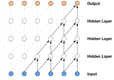
A Temporal Convolutional Network (TCN) is a model architecture composed of stacked residual blocks, where each block utilizes dilated causal convolutions.
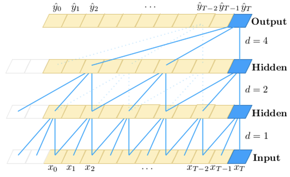
A key feature is the use of increasing dilation factors in successive layers. As the network deepens, the receptive field grows exponentially, this allows the model to efficiently capture long-range dependencies and “see” a large portion of the input sequence without requiring an excessive number of layers.
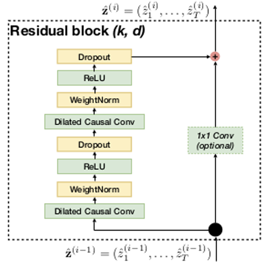
Similar to how architectures like VGG are built from blocks, a TCN is composed of these residual blocks. Each individual block contains a small pipeline that is typically applied twice:
- A dilated causal 1D convolution (with a specific kernel size , e.g., ).
- Weight Normalization (used to stabilize and speed up training by decoupling weight direction from magnitude).
- ReLU activation (for non-linearity).
- Dropout (for regularization to reduce overfitting).
After this two-layer pipeline, a residual connection (or skip connection) adds the original input of the block to the block’s final output. If the input and output have different dimensions (e.g., due to a change in the number of filters), a 1x1 convolution is applied to the input (on the skip connection) to match its shape before the addition
TCN VS RNN
Temporal Convolutional Networks (TCNs) can outperform recurrent models like LSTMs and GRUs on a wide range of sequence modeling tasks.
Their appealing properties, when compared to RNNs, include:
- Parallelism: TCNs are highly parallelizable. Unlike RNNs, which must process data sequentially (where the output at time depends on the computation from ), the convolutions in a TCN can be computed in parallel across the entire sequence. This results in significantly faster training, especially on long sequences.
- Stable Training: TCN training is generally more stable as the backpropagation path is not sequential, which avoids the vanishing and exploding gradient problems common in RNNs.
- Higher effective memory: the “memory” (or receptive field) of a TCN is explicitly controlled by the network’s depth and dilation factors (). This allows the model to efficiently capture very long-range dependencies. In contrast, an RNN’s memory is tied to its hidden state, and attempting to capture long dependencies often leads to gradient instability during backpropagation through time.
- Explainability: Since TCNs are fundamentally convolutional networks, they are compatible with standard CNN explainability tools. Methods like Grad-CAM (Class Activation Maps) can be used to generate activation maps, providing insights into which parts of the input sequence (or which features) were most important for a given prediction.
Transformer
FROM TEMPORAL CONVOLUTIONS TO TRANSFORMERS
Temporal Convolutional Networks (TCNs) model temporal dependencies using a fixed inductive bias: local convolutions with an expanding receptive field. This means that the model processes data along the temporal axis in order, enforcing causality — what happens in the past influences what happens in the future, and never the other way around.
This inductive bias is powerful, as it ensures stability and causal consistency, but it may not always be the best assumption for every problem. In some cases, relevant information is non-local in time, meaning that an item can depend on elements that are very distant in the sequence or follow long-range dependencies that do not obey a strict temporal order.
Example: Code Understanding
In source code, the opening of a for loop or a bracket { may influence variables or a corresponding closing bracket } dozens of lines later. This creates a long-range dependency that is difficult for a model based on local convolutions to capture.
TRANSFORMER ARCHITECTURE
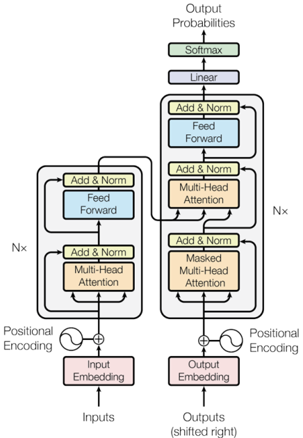
The solution are the so-called attention-based models or transformers. This architecture is composed of two main components:
- Encoder — on the left in the figure
- Decoder — on the right in the figure
Both the encoder and decoder consist of a stack of identical layers (or “blocks”), typically with , forming a deep architecture capable of capturing complex and long-range dependencies within the data.
Transformers have become ubiquitous across AI applications:
- Machine translation and text generation
- Question answering and dialogue systems
- Computer vision (Vision Transformer, ViT)
TRANSFORMER ENCODER
A Transformer encoder block receives an input sequence of tokens — for example, tokens, each represented by a vector of dimension — and produces an output sequence of the same shape.
No pooling or dimensionality reduction is applied: the encoder preserves the sequence length and dimensionality, but transforms the content of each token as it passes through the layers.
This is in contrasts with CNNs, which often change the dimensions (e.g., feature/channel size) of their input.
Each encoder block is composed of the following main components:
- A Multi-Head Attention (MHA) layer (detailed later).
- Add & Norm:
- A Residual (skip) connection is applied, adding the input of the MHA layer to its output, to facilitate gradient flow.
- Layer Normalization is applied to the result.
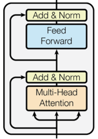
-
A Feed-Forward Neural Network (FFN), a simple MLP applied independently and in parallel to each token embedding. Typically is composed of two linear layers with a ReLU activation in between.
The standard design first expands the dimensionality and then contracts it back to the original size:
- Layer 1 (Expand):
- ReLU Activation
- Layer 3 (Contract):
Where is the “feed-forward” inner dimension, often set to .
-
Add & Norm:
- Another Residual connection adds the input of the FFN to its output.
- Layer Normalization is applied again.
Layer Normalization
Layer Normalization (LN) is a technique used to stabilize and speed up training.
Unlike Batch Normalization, which normalizes activations across the batch dimension, Layer Normalization operates across the feature dimension — i.e., it normalizes the features within each individual sample (token).
Given an input vector representing one token with features, computes:
where:
- → is the mean of the features of the token
- → is the variance over the features
- → learnable parameters that allow the model to rescale and shift the normalized output
- → small constant for numerical stability
Thus, normalization is applied per token, not across different tokens in the same batch.
In Transformers, Layer Normalization is applied multiple times throughout both the encoder and decoder stacks — typically after each residual connection — ensuring that at every layer, the activations maintain a stable scale and distribution.
Multi-Head Attention
THE CORE IDEA OF ATTENTION
In many sequence tasks, not all input elements are equally relevant for producing a given output. Traditional models (like RNNs or CNNs) process information uniformly or with a fixed receptive field, which limits their ability to focus on what truly matters.
Attention solves this problem by allowing the model to dynamically assign “importance” weights to different input elements based on their relevance to the current context. At each step, the model effectively asks: “Which tokens should I pay more attention to right now?”
Given an input sequence of tokens, , the attention mechanism produces a new sequence of contextualized representations:
where each output vector is a weighted combination of all input vectors .
The attention coefficients are not fixed. They are learned functions of the input, computed through dedicated parametric modules. Thus, the model learns where to look depending on the specific input sequence.
For example, to create , the model might learn that it is composed of 80% information from , 10% from , and 10% from .
ATTENTION AS CONTENT-BASED MEMORY ACCESS
Instead of compressing all contextual information into a single hidden state (as done in RNNs), the attention mechanism allows the model to directly query the entire sequence of inputs and retrieve the most relevant information on demand.
This process functions as a form of content-based memory access, where retrieval depends on what is stored, not where it is stored.
The model maintains a set of memory slots constructed from the entire input sequence . For each token , the model generates two vectors:
- Key (): Acts as an “index” or “label.” It represents what kind of information this token offers (e.g., “I am a subject,” “I am a verb”).
- Value (): Represents the token’s actual content or what information it provides.
The complete set of pairs constitutes the memory.
To retrieve information, the model generates a Query vector , which describes what the model is looking for. This query is used to retrieve the most relevant information from the memory by computing a weighted combination of all values .
The weights are determined by computing the similarity between the query and each corresponding key , as formalized in the algorithm below.
Algorithm 2 Content-based Retrieval
Require: query , keys , values
for each memory slot do
end for
— attention weights
— retrieved information
return
QUERY, KEYS AND VALUES
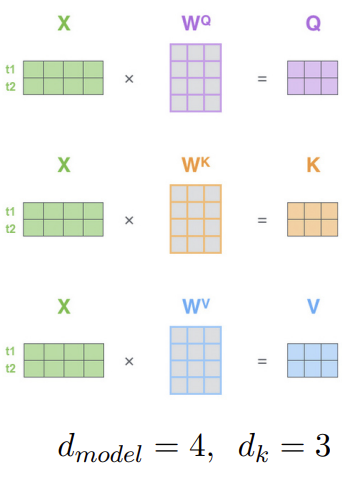
In the attention mechanism, the Query , Key , and Value matrices are generated by projecting the entire input sequence through three distinct, trainable linear layers (weight matrices):
The input tokens are projected into a new dimension , following these relationships:
- Input → The input sequence matrix consists of tokens and has the shape
- Weights → Each weight matrix maps the input dimension to the new one and therefore has shape .
- Output → The resulting matrices all share the shape . Each row corresponds to the respective vector of a token — for example, the first row represents for the first token, the second row represents for the second token, and so on.
Since all three components originate from the same input , the attention mechanism is referred to as self-attention.
SINGLE-HEAD ATTENTION
This mechanism acts as a form of content-based memory access: the model can look back at all inputs and retrieve information on demand.
Where are the matrices representing Queries, Keys, and Values, respectively. The calculation involves four steps:
-
Compute Similarity Scores
The dot product produces a similarity matrix where the entry measures how much every token (query) is similar to token (key).
Shape:
-
Scale
To stabilize the gradients, the scores are scaled by dividing by
A typical value for the dimension is
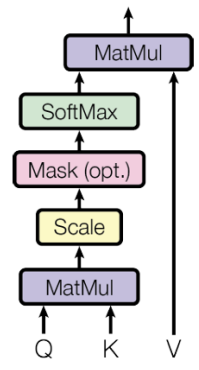
-
Normalize (Softmax)
To convert the raw scaled scores into attention weights (which sum to 1), a softmax function is applied to each row (row-wise) of the scaled score matrix. Let’s call this resulting attention matrix .
-
Compute Weighted Sum
Finally, the attention weight matrix is multiplied by the Value matrix :
Shape:
The result is the new output matrix, where each row is the new representation of token , computed as a weighted sum of all value vectors in the sequence.
MULTI-HEAD ATTENTION
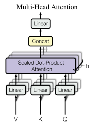
In multi-head attention the linear projections and the attention are repeated in parallel multiple times (e.g., ), each using a distinct set of weights.
Each head produces an output of dimension , and the resulting outputs are concatenated along the feature axis. The concatenated vector is then projected through a final linear layer to restore the dimensionality of
where:
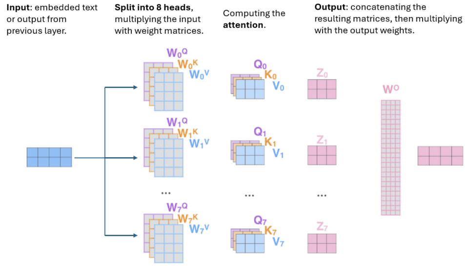
FROM TOKEN REPRESENTATION TO CLASSIFICATION
The encoder produces a sequence of token embeddings, where each vector represents a contextualized version of its corresponding input token.
To perform classification, this sequence must be reduced to a single, fixed-size representation. Two common strategies are:
-
Average pooling: Compute the mean of all token embeddings and use the resulting vector as input to a Multi-Layer Perceptron (MLP) classifier:
This produces a single feature vector with the same dimensionality as the original embeddings. The MLP then maps this vector to the number of output classes through a final linear layer.
-
[CLS] token: Introduce a special classification token prepended to the input sequence. Its embedding, , after passing through the encoder, serves as a global representation of the entire sequence.
The [CLS] embedding is then fed into an MLP for classification, while the remaining token embeddings are discarded.
SUMMARY
Both Temporal Convolutional Networks (TCNs) and Transformers are powerful architectures for modeling sequential data, but they rely on different inductive biases and computational mechanisms. While TCNs are based on convolutional operations, Transformers use attention to model dependencies between sequence elements. The following table summarizes their main differences and characteristics:
| Aspect | Temporal Convolutional Networks (TCNs) | Transformers |
|---|---|---|
| Modeling Mechanism | Use causal and dilated convolutions to capture temporal dependencies. | Use attention mechanisms to model relationships between all elements in a sequence. |
| Temporal Coverage | Capture local-to-mid-range temporal structures efficiently. | Learn arbitrary long-range dependencies with no fixed receptive field. |
| Training Stability | Generally stable and easy to train due to convolutional nature. | Training can be more complex but allows greater flexibility. |
| Context Handling | Best suited for sequential and time-ordered data. | Naturally handle multimodal and non-sequential contexts. |
| Applications / Influence | Effective for tasks with structured temporal signals (e.g., time series). | Serve as the foundation of modern architectures like BERT, GPT, and ViT. |
Loss Function for Regression
CLASSICAL REGRESSION LOSSES
-
Mean Squared Error (MSE)
- Penalizes large errors quadratically: This characteristic makes the loss function highly sensitive to outliers.
- Reduces small errors: Conversely, if an error is small (), squaring it makes it even smaller (e.g., ).
- Optimization: The function is smooth and continuously differentiable, making it stable and well-suited for gradient-based optimization.
-
Mean Absolute Error (MAE)
- Robust to outliers: It penalizes all deviations linearly.
- Optimization: The function is not differentiable at zero (it has a “kink” or a discontinuous gradient). This can lead to instability during the training and optimization process, especially when using standard gradient-based methods.
FROM REGRESSION TO CLASSIFICATION VIA BINNING
By discretizing a continuous target variable into intervals (bins), we can transform a regression problem into a classification one and train the model using a cross-entropy loss to predict which interval the target value belongs to.
Age Prediction from an Image
- Target variable (Regression): age
- Target variable (Classification): Define bins, e.g.:
- Class 1: [0–10]
- Class 2: [10–20]
- …
- Class 10: [90–100]
- Train a classifier with output classes (one per age interval)
- The final prediction can be the center of the predicted bin (e.g., 25 for the [20–30] bin) or, more robustly, a weighted average of all bin centers based on the output class probabilities.
It is particularly useful when small variations in the target value are not critical, and the main interest lies in the broader range or category of the prediction.
Classification problems are often easier to optimize than regression ones, since the loss function provides a stronger and more focused learning signal through the softmax output — the gradient clearly points toward the correct class.
LIMITATIONS OF MSE AND MAE
Both Mean Absolute Error (MAE) and Mean Squared Error (MSE) assume symmetric errors, meaning that overestimation and underestimation are penalized equally.
However, in many real-world scenarios, this assumption is not appropriate:
- The cost of underpredicting can differ significantly from that of overpredicting (e.g., in energy demand, risk assessment, or stock forecasting).
- In some cases, we are not interested in predicting a single “average” value, but rather in estimating a range of possible outcomes.
For example, with MSE, an error of +10 and an error of –10 contribute equally to the loss, since the sign is lost when squaring the difference. This symmetry ignores situations where one type of error is more critical than the other.
To address this limitation, we can use the Quantile Loss.
QUANTILES
The -quantile of a probability distribution is the value such that a random variable from the distribution will be less than or equal to with probability :
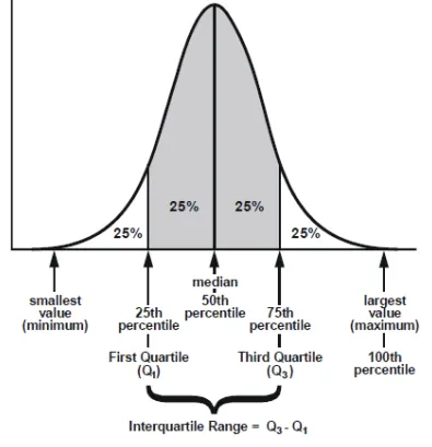
-
(90th percentile):
is the value such that 90% of the observations are below it and 10% are above.
If the 90th percentile of exam scores is 85, it means 90% of students scored below 85.
-
(median):
The median is the 0.5 quantile — half the observations are below it, half above.
In the ordered set [1, 3, 5, 7, 9], the median is 5.
-
(10th percentile):
is the value such that 10% of the data is below it and 90% above.
In income data, the 10th percentile is the income level below which the poorest 10% of people fall.
QUANTILE LOSS
The Quantile Loss allows the model to estimate specific quantiles of the target distribution, rather than just the mean. This introduces asymmetry in the loss, because the penalty for overestimation and underestimation depends on the chosen quantile .
Properties:
- is the target, while is the estimate.
- is a hyperparameter that controls which quantile we want to estimate.
- median (50th percentile)
- 90th percentile (upper bound)
- 10th percentile (lower bound)
Intuition
By adjusting , we can control how much the model penalizes one side of the error:
- For : underestimations are penalized 9× more than overestimations → the model prefers to slightly overpredict.
- For : overestimations are penalized 9× more → the model prefers to underpredict.
- For : both sides are penalized equally → same as MAE.
The model “pays” more for errors on one side of the prediction, depending on the chosen quantile .
Key Takeaways
| Topic | Key Point |
|---|---|
| 1D Convolution | Adapts CNN convolutions to sequential data by sliding a kernel along the temporal axis |
| Dilated Convolution | Introduces gaps between kernel elements to exponentially expand the receptive field without adding parameters |
| Causal Convolution | Ensures output at time depends only on inputs , enforcing temporal causality |
| TCN | Stacks residual blocks with dilated causal convolutions; parallelizable and stable vs. RNNs |
| Transformer | Encoder–decoder architecture using attention instead of convolutions to model arbitrary long-range dependencies |
| Self-Attention | Each token queries all others via Q, K, V projections; computes weighted combinations based on content similarity |
| Multi-Head Attention | Runs multiple attention heads in parallel, then concatenates — captures diverse relational patterns |
| Layer Normalization | Normalizes per-token features (not across the batch) to stabilize training in deep transformers |
| MSE vs MAE | MSE penalizes outliers quadratically; MAE is robust but non-differentiable at zero |
| Quantile Loss | Asymmetric loss that estimates specific quantiles of the target distribution, useful when over/underprediction costs differ |