Transfer Learning
Introduction
Transfer learning involves reusing a model trained on a source task in a data-rich domain to improve performance on a different (downstream) task in a data-scarce domain. Rather than training from a random initialization, the model begins with pretrained weights. This allows the model to transfer previously acquired knowledge, such as linguistic structures or visual patterns, to the new application.
ADDRESSING DATA SCARCITY AND OVERFITTING
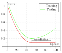
Transfer learning is essential when the target task has limited data. Training deep models with millions or billions of parameters on small datasets often leads to overfitting, where the model learns specific training data patterns that do not generalize to unseen data. A typical sign of overfitting is that training error continues to decrease while validation or test error increases.
This situation can be viewed as epistemic uncertainty, which arises from insufficient knowledge or data to determine reliable parameter values. However there are three primary strategies to mitigate this uncertainty and improve model generalization:
-
Collect more data:
Collecting more data is almost always the most effective option, particularly when data exhibits high variability or significant intra-class differences. However, this is often expensive or infeasible in specialized domains like medical imaging or rare event detection.
-
Regularization techniques
Regularization encourages the development of simpler models that generalize better. Common methods include:
- Weight decay (L2 regularization)
- Dropout, data augmentation
- Early stopping
- Model pruning/shrinking
-
Introduce inductive bias
This involves injecting prior knowledge or structural assumptions into the model to guide learning. Transfer learning itself is one form of inductive bias.
INDUCTIVE BIAS
Inductive bias is the set of prior assumptions or constraints built into a learning algorithm to guide its generalization. Its main job is to reduce the “hypothesis space,” helping the model to favor specific hypotheses over other when multiple patterns fit the data. This is crucial when training data is scarce, as it prevents the model from getting lost in infinite possibilities.
Formal Definition
The inductive bias of a learning algorithm is the set of assumptions that uses to select one hypothesis from all consistent options:
Equivalently, can be viewed as:
- A restriction of the hypothesis space (restriction bias)
- A preference ordering over hypotheses (preference bias)
Examples:
- Convolutional Neural Networks: Assume locality and translation invariance, meaning nearby pixels are correlated and local patterns are meaningful regardless of their position in the image.
- Graph Neural Networks: Use an adjacency matrix to encode structural priors about the relationships within a specific domain.
- Sparse Autoencoders: Operate on the assumption that sparse representations are more likely to capture meaningful semantic features.
- Transformers: Impose fewer domain-specific assumptions, relying instead on attention mechanisms to learn relationships. Because they possess weaker inductive biases than CNNs or GNNs, they typically require massive datasets to perform well.
INDUCTIVE BIAS IN TRANSFER LEARNING
Transfer learning serves as a powerful form of inductive bias. It operates on the fundamental assumption that a model trained on a large, related source domain has already learned representations useful for the target task. In other words, pretraining on a source domain provides a parameter initialization () close to an optimal solution () for the target domain.
The pretrained model acts as a strong prior, significantly reducing epistemic uncertainty in scenarios where data is scarce.
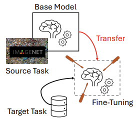
Fine-Tuning
The standard transfer learning pipeline is organized into two primary stages:
-
Pretraining on a source task
A model is trained on a large dataset and learns a set of weights representing general features.
-
Fine-tuning on a target task
The pretrained weights are used as the initialization for the model, which is then further trained on the target dataset to slightly adjust the parameters. Since many useful features are already learned during pretraining, the target model requires significantly less data and fewer parameter updates.
Example Include:
- Computer Vision
- Pretrain a CNN on ImageNet (source task).
- Obtain a set of learned weights that recognize edges, textures, and shapes.
- Use these weights as initialization for training on a new task (fine-tuning) e.g., fine-tune for medical image classification.
- Natural Language Processing (NLP):
- Pretrain a language model on a wide corpus, such as Wikipedia, to learn linguistic structures.
- Fine-tune it for sentiment analysis.
BEYOND FINE-TUNING
Fine-tuning is a common way to transfer knowledge from a source model to a target task, but it is not the only one. Other approaches:
- Knowledge Distillation (to be covered later): Transfer knowledge from a teacher model to a student model using soft targets.
- Domain Transfer: the general case in which source and target domains may differ in sample space, label space, data distribution, or all of them (e.g., moving from natural images to medical images).
- Domain Adaptation: a specific case where sample and label spaces remain the same and only the data distribution changes (e.g., detecting the same objects under different visual conditions).
In all cases, the goal is to leverage prior knowledge to reduce data requirements and improve generalization.
WHY FINE-TUNING IS DOMINANT IN PRACTICE
Fine-tuning has become the standard approach because it offers several advantages:
- Performance: Fine-tuning often outperforms training from scratch, especially in data-scarce scenarios.
- Computational constraints: Training very large models from scratch is prohibitively expensive for most organizations.
- Data availability: The large datasets required for full training are not always accessible.
- Reuse: Many frameworks provide pretrained weights that can be adapted with minimal additional training. This avoids the massive computational cost of pretraining and reduces the time-to-market for deploying models.
- Reduced design effort: Pretrained models come with well-tested architectures and hyperparameters validated through extensive research and benchmarking, allowing practitioners to focus on the target task rather than low-level model design.
EFFECTIVENESS OF FINE-TUNING
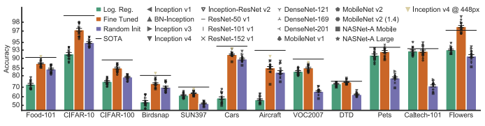
The comparison illustrates performance across three approaches:
- Logistic regression (green)
- Fine-tuning (red)
- Training from random initialization (purple)
The accuracy bars show that, across these architectures, fine-tuning achieves the best performance.
Key Advantages of Fine-Tuning
- Superior Accuracy: Models using pretraining generally outperform those trained from scratch, with the gap most evident on small datasets.
- Data Scaling: Although training from scratch can approach similar performance with very large datasets, fine-tuning is more effective when data is limited.
- Faster Convergence: Even when final accuracy is similar, pretrained models converge much faster because they start from meaningful features rather than random weights.
Technical Aspects of Fine-Tuning
FREEZING LAYERS
Earlier layers often capture generic low-level features (e.g., edges, textures, simple patterns) that can be reused across tasks, while deeper layers become increasingly task-specific. For this reason, a common strategy during fine-tuning is to freeze layers capturing general features and retrain those responsible for higher-level representations.
Freezing layers during fine-tuning provides several benefits:
- Reduced computation: Frozen layers can be set to
no_grad, lowering memory consumption and avoiding gradient computations. - Preserved generalization: Maintains robust low-level features learned in the source task, reducing the risk of overfitting the target dataset.
- Faster convergence: The optimizer updates only task-specific layers, requiring fewer parameter changes.
- Stability: Prevents useful pretrained representations from being distorted
Conversely, updating the entire model forces all parameters to readapt, increasing training time and the risk of overfitting.
LAYERS TRAINED DURING FINE-TUNING
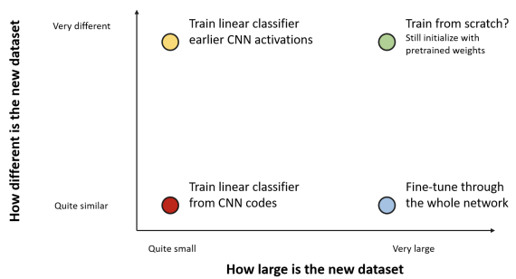
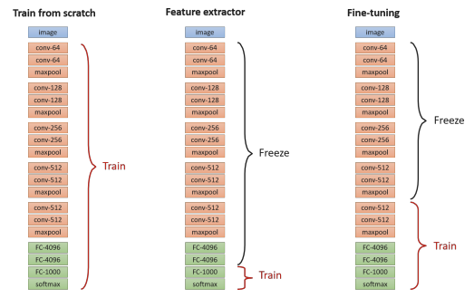
When adapting a pretrained model to a new task, deciding which layers to update is critical. Three main strategies are commonly used:
- Linear Probing (Feature Extraction): All pretrained layers are frozen, and only the classification head is trained (the last layer). In this setup, the network functions exclusively as a fixed feature extractor, so the optimization process focuses solely on learning the final mapping to the target classes. This approach offers fast adaptation and a low risk of overfitting but provides limited flexibility as it relies entirely on the features learned during the original pretraining.
- Fine-Tuning: Some pretrained layers are unfrozen so the model can adapt its learned representations This can be done in two ways:
- Partial Fine-Tuning (Last layers): Only the deeper, more task-specific layers are updated, balancing adaptation capacity with computational efficiency.
- Full Fine-Tuning (All layers): The entire network is updated. This offers maximum flexibility and performance but requires more data and higher computational costs to avoid overfitting.
- Training from Scratch: All weights are initialized randomly, requiring the model to learn every feature representation from zero.
Note: Linear probing is often used in the literature as a baseline — a quick way to evaluate how well the features learned by a frozen backbone transfer to a downstream task. If a more sophisticated fine-tuning strategy fails to outperform it, the transfer learning approach is likely ineffective.
LEARNING RATE STRATEGIES DURING FINE-TUNING
Fine-tuning generally requires smaller learning rates () than training from scratch to avoid to alter pretrained features. Because different layers play different roles, several learning-rate strategies are commonly used:
- Uniform learning rate: Apply the same learning rate to all trainable layers.
- Pros: Simple to implement.
- Cons: Often suboptimal, as it may over-update early layers (destroying generic features) or under-update task-specific layers.
- Layer-specific learning rate: Commonly known as the “Slow Learner” technique, this involves assigning smaller learning rates to earlier layers and larger rates to later, task-specific layers. This preserves generic low-level features while allowing high-level representations to adapt more quickly to the new task.
- Warmup schedules: Training begins with an extremely small learning rate that gradually increases over the initial iterations before reaching its peak or beginning a decay. This is particularly critical when updating the entire network (Full Fine-Tuning).
Using excessively large learning rates during fine-tuning can cause catastrophic forgetting, where pretrained knowledge is rapidly overwritten.
AN ALTERNATIVE: LP-FT
Standard fine-tuning can sometimes distort pretrained features, leading to low performance on out-of-distribution (OOD) data. This happens because the model may over-specialize to the target dataset and lose the general knowledge learned during pretraining.
In contrast, Linear Probing (LP) keeps the pretrained backbone frozen, preserving general features and often improving robustness to distribution shifts. To capture the benefits of both methods, a hybrid strategy known as LP-FT (Linear Probing Fine-Tuning) is often employed.
The Two-Stage Process:
- Stage 1 (Linear Probing): The pretrained backbone is frozen, and only the linear classifier is trained to convergence.
- Stage 2 (Fine-Tuning): The entire network is unfrozen and fine-tuned, starting from the weights obtained in the probing stage.
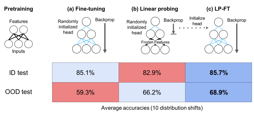
Why this works?
LP-FT works because linear probing first finds a strong classifier on top of fixed, stable features. Subsequent fine-tuning then refines these features in a controlled way, rather than drastically altering them.
BATCH NORMALIZATION IN FINE-TUNING
In many transfer learning scenarios, the Batch Normalization (BatchNorm) layers are updated even when the rest of the model’s weights remain frozen. This is because BatchNorm layers store dataset-specific statistics — running mean and running variance — that must be aligned to the target domain to prevent performance drops caused by distribution mismatch.
Only the internal running statistics are recomputed to match the new data distribution. The learnable parameters, (scale) and (shift), can either be fine-tuned or kept fixed.
This process is functionally equivalent to running a single training epoch with a learning rate of . No weights are modified; only the internal normalization statistics adapt.
This process adapts normalization to the new domain without altering the learned features, effectively aligning source and target feature distributions. This is a foundational practice in domain adaptation.
LIMITATION OF FINE-TUNING
Despite its effectiveness, fine-tuning presents several practical and methodological limitations:
-
Architectural rigidity: Fine-tuning constrains the target task to the architecture of the pretrained model, which may not be optimal. For example, a model with too many layers creates unnecessary computational overhead for simpler tasks.
-
Inherited biases: Pretrained models inherit biases from their source datasets. A well-known example is the texture bias observed in many CNNs:
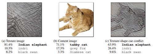
Models tend to rely more on local texture patterns rather than on global shape information. In cue-conflict scenarios — for instance, an object with the shape of a cat but the texture of elephant skin — the model may classify the object based on texture rather than shape, revealing a limitation in learned representations.
-
Dependence on external data/models Fine-tuning relies on the availability of high-quality pretrained models and their associated datasets. This includes potential licensing or usage restrictions.
-
Large storage requirements: Fine-tuning updates the entire set of model parameters. For large models like Large Language Models (LLMs) this is a significant logistical challenges in terms of:
- Memory Footprint Each downstream task requires storing a separate full model copy.
- Deployment Costs: Maintaining multiple versions of the same base model is expensive.
- Resource Constraints: Switching tasks on memory-constrained devices becomes difficult.
SUMMARY
Key technical aspects:
- Layer selection: train last layer(s) or the whole network.
- Freezing layers: preserve generic low-level features, reduce computation.
- Learning rate strategies: single LR vs. layer-specific (discriminative) LR, warmup.
- BatchNorm handling: freeze weights, update statistics, or fully train.
Advantages:
- High performance with limited target data.
- Lower computational cost than training from scratch.
- Faster convergence, lower time-to-market.
Limitations:
- Dependence on external pretrained models and datasets (e.g., license).
- Inherited biases from the source domain.
- Large storage requirements for multiple fine-tuned variants.
Teacher-Student Approaches
THE IMPACT OF DEPTH
Teacher–student approaches are motivated by the observation that, in a high-data regime, increasing the depth of a neural network generally improves performance. Deeper models can learn hierarchical feature representations and capture more complex patterns, leading to better accuracy.
DEEP ENSEMBLES FOR MODEL UNCERTAINTY
A similar effect appears in deep ensembles, where multiple independent models are trained using different random initializations and data shuffling. While each model converges to a different local minimum, all remain consistent with the training data.
Their disagreement reflects epistemic uncertainty:
- If all models agree high confidence.
- If models disagree high uncertainty.
Both deep models and ensembles improve robustness and performance through redundancy. However, their large size leads to high computational and memory costs, making deployment difficult on resource-constrained platforms.
While both deep models and ensembles improve robustness and performance through redundancy, they face significant practical limitations. Their large size results in high computational and memory requirements, making them difficult to deploy on resource-constrained platforms like embedded systems, robots, or edge devices.
Since constraints on computation and memory footprint are far more severe at test time than during training, we require a method to transfer the knowledge from these large, high-performing models into smaller, more efficient ones. This principle is formalized as knowledge distillation.
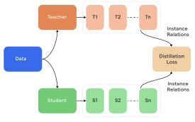
Knowledge Distillation
The core objective of knowledge distillation is to train a smaller student model to mimic the output distribution of a larger teacher model, rather than attempting to replicate its specific architecture.
The Model Roles:
- The Teacher: A large, complex model or an ensemble of models (whose prediction are averaged) trained on the target task without architectural constraints. It serves as the high-performing reference.
- The Student: A smaller, more efficient model designed to meet specific deployment constraints while approximating the teacher’s input-output mapping.
SOFTENED PROBABILITY
During standard training, the teacher produces logits for each class . Using the standard softmax, the predicted class typically receives a probability close to one, while the others are near zero.
To transfer richer information, a temperature parameter is introduced in the softmax during training:
Increasing produces a softer probability distribution:
- Lower confidence in the top class.
- Higher probabilities for classes the teacher considers similar.
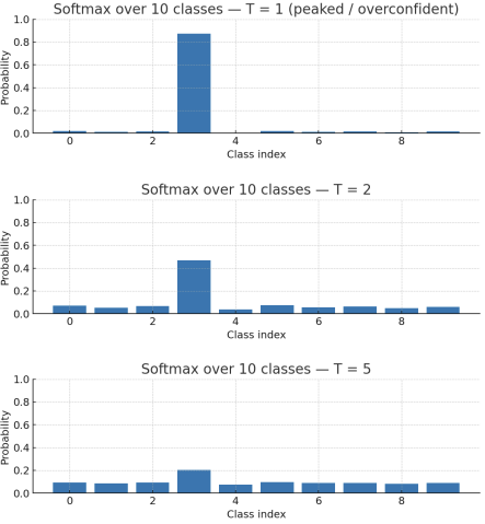
As increases, the probability spreads across more classes, revealing information about inter-class relationships (dark knowledge) learned by the teacher.
At inference time, is set back to 1.
TRAINING PROCEDURE
- Teacher Forward Pass: Obtain teacher logits .
- Student Forward Pass: Obtain student logits .
- Loss Calculation: Update student parameters using a weighted combination of two losses:
- Fidelity to Ground Truth: Standard cross-entropy loss () with respect to the ground-truth labels .
- Fidelity to Teacher (Distillation Loss): Cross-entropy (or KL divergence) using the softened teacher probabilities.
Where:
- : ground-truth one-hot label
- : softmax function
- : temperature ( during distillation)
- : weight balancing hard vs. soft targets
DARK KNOWLEDGE
The effectiveness of knowledge distillation is driven by dark knowledge: the information contained in the relative probabilities of the non-argmax classes (the secondary information).
As we said before, while a standard label only identifies the correct class, dark knowledge reveals the class similarity structure learned by the teacher. When the temperature is increased, these secondary relationships become visible, allowing the student to capture how classes relate to each other.
Consider an image of a Cat. A one-hot label only provides “Cat.” However, the teacher might output:
This distribution tells the student that a cat is more similar to a dog than to a fox. These secondary probabilities can guide the student to learn richer decision boundaries than one-hot labels allow.
In some cases, the student can achieve performance comparable to, or even slightly better than, the teacher. This is because the student benefits both from the teacher’s structured knowledge (via distillation) and from direct supervision through ground-truth labels.
Soft targets also act as a strong regularizer, preventing the model from becoming overconfident. The teacher’s signal further contributes to regularization, as it reflects a stable representation that typically does not overfit.
ALTERNATIVE: DISTILLATION VIA PRE-SOFTMAX ACTIVATIONS
Instead of matching softened output probabilities, distillation can be performed with logit matching by directly aligning the teacher and student pre-softmax activations (logits) using Mean Squared Error (MSE).
Given the teacher logits and student logits , the loss for classes is defined as:
This approach can be combined with standard cross-entropy to ground-truth labels to maintain accuracy.
Advantages:
- Avoids potential information loss introduced by the softmax transformation.
- Emphasizes the transfer of secondary information about class similarities learned by the teacher.
APPLICATIONS OF KNOWLEDGE DISTILLATION
- Model compression: Reduce memory footprint and computational cost for deployment on edge devices or mobile platforms.
- Ensemble-to-single transfer: Replace a large ensemble with a single student model trained to approximate the ensemble’s aggregated predictions.
- Cross-architecture transfer: Since distillation focuses on the functional mapping (input-output) rather than the internal structure, knowledge can be transferred between different architectures—such as distilling a Transformer into a CNN (or vice versa) to leverage specific hardware strengths.
- Domain adaptation: Transfer knowledge from a teacher trained in one domain to a student in a related but different domain.
- Regularization in training: Use self-distillation to improve generalization by making a model learn from its own earlier predictions.
Beyond Vanilla Knowledge Distillation
SIMILARITY-PRESERVING KNOWLEDGE DISTILLATION
Similarity-Preserving Knowledge Distillation (SP KD) instead of matching only the output logits of teacher and student, also preserve the pairwise similarities between samples in the feature space. Instead of focusing only on the final predictions, it leverages internal feature activations.
Motivation The relational structure among data points in the embedding space contains information that individual predictions do not capture. By maintaining these relationships, the student learns the underlying teacher’s feature representations.
Procedure
-
Compute Similarity Matrices:
For a batch of samples, compute the (Teacher) and (Student) similarity matrices from their internal features.
-
Minimize Distance: In addition to the standard KD or cross-entropy loss, minimize the difference between these matrices, typically using the Frobenius norm:
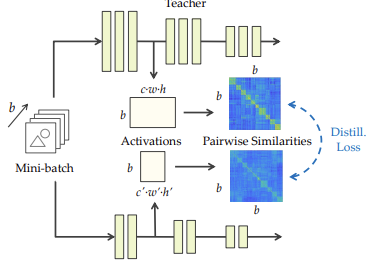
This enforces that the student preserves the relational structure between samples learned by the teacher.
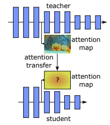
ATTENTION TRANSFER
Attention Transfer (AT) is a distillation technique where the student is trained to mimic the teacher’s spatial attention maps rather than just its raw activations or output probabilities. This approach teaches the student not only what to predict, but also where to look within the input data.
Procedure
- Extract Attention Maps: From teacher and student feature maps , compute attention maps and by aggregating across channels :
where:
- is the -th feature channel
- (typically for norm).
- Normalize each attention map to unit norm.
- Minimize: Use the distance between the normalized maps:
- Combine Losses Integrate with standard Cross-Entropy (CE) or Knowledge Distillation (KD) loss.
Interpret the Attention Map
The attention map is a single-channel map:
- High Value: Indicates a spatial region strongly activated across many channels (highly informative).
- Low Value: Indicates regions with little activity.
The objective is to encourage the student to focus on the same spatial regions as the teacher.
Benefits and Limitations:
- Architectural Flexibility: AT improves transferability even when the teacher and student differ in depth or structure.
- Dimensional Alignment: If spatial dimensions differ, linear projections or up/down-sampling are required to align the maps.
- Layer Matching: Corresponding layers can be chosen flexibly, but the hierarchical order should be preserved (e.g., early layers matched with early layers).
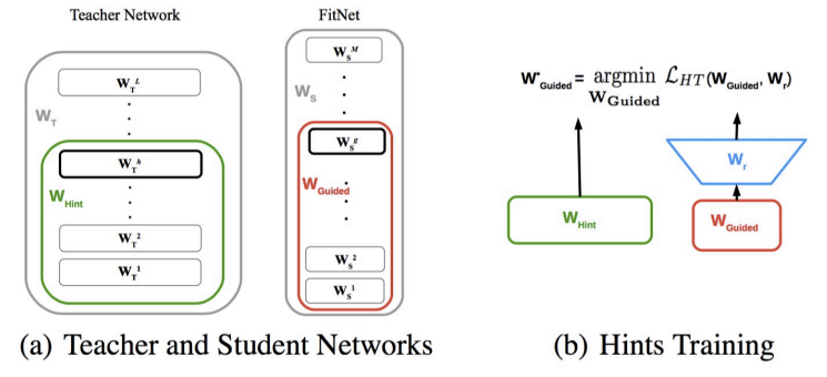
FITNETS: HINTS FOR THIN DEEP NETS
FitNets extends standard knowledge distillation by transferring intermediate feature representations from the teacher to the student, rather than focusing solely on final output logits.
Motivation
Training a very deep but thin student network from scratch can be challenging due to convergence issues. Providing intermediate “hints” from the teacher’s internal layers helps guide the student’s learning process.
Procedure
- Layer Selection: A hint layer is selected from the teacher, and a corresponding guided layer is selected from the student.
Coherent Matching: Layers must be aligned by relative depth. You must avoid “cross-matching” (e.g., matching a shallow student layer to a deep teacher layer) to preserve the hierarchical structure of representations.
- Dimensional Alignment: If the feature map dimensions or channel counts differ, a small regressor (such as a convolution or MLP) is added to map the student’s guided layer to the teacher’s hint layer dimensions.
- Loss Calculation: In addition to standard KD loss, FitNets minimizes the Mean Squared Error (MSE) between the mapped student features and the teacher features :
Choosing Layers and Architecture
There is no strict rule for layer selection, as it depends heavily on the specific architecture. Typically:
- A deep intermediate layer of the teacher serves as the hint.
- A student layer at a comparable depth serves as the guided layer.
FitNets is particularly effective because it is not restricted to teacher-student pairs of the same size. It excels even when:
- The student is deeper but thinner than the teacher.
- The student is shallower with a different architecture.
- The hidden layer sizes differ (the regressor handles the dimensionality shift).
SELF-KNOWLEDGE DISTILLATION
Self-Knowledge Distillation applies the distillation framework between two networks with the same architecture. In this setup, the primary difference between the teacher and the student lies in the quality or type of input information rather than the model size.
Procedure
- Initial Training: Train a teacher model on richer, more informative, or complete inputs.
- Distillation Phase: Use that trained model as a teacher to guide a second instance of the same architecture (the student) from scratch on degraded, partial, or noisier versions of that same data.
- Optimization: The student minimizes a distillation loss that combines standard supervision with the teacher’s guidance, which allows the student to match the teacher’s intermediate features or final predictions.
Key Benefits and Intuition
- Input Efficiency: Shifts the learning challenge from increasing model capacity to improving input efficiency.
- Performance Gains: Even when architecture and data are identical, students often achieve a 2–3% improvement over the teacher, as the teacher acts as an additional regularization signal, helping organize the feature space and extract more discriminative patterns.
- Cross-Modality Learning: Useful when some input modalities are missing or only partial observations are available.
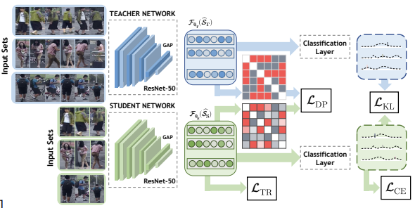
Application of Self-KD:
In this Self-Knowledge Distillation application, a teacher model is trained on full video sequences to recognize individuals, while a student model receives only a subset of frames. Through distillation, the student learns to interpolate missing frames and approximate the teacher’s outputs, extracting rich temporal and spatial cues from limited data.
Conclusions
- When extracting knowledge from data we do not need to worry about using very big models or very big ensembles of models that are much too cumbersome to deploy.
- If we can extract the knowledge from the data it is quite easy to transfer most of it into a much smaller model for deployment.
- KD enables a separation of concerns: train for accuracy, deploy for efficiency.
Key Takeaways
| Concept | Description |
|---|---|
| Transfer learning | Reuse weights pretrained on a data-rich source task to bootstrap a data-scarce target task; mitigates overfitting and epistemic uncertainty |
| Inductive bias | Prior assumptions baked into the algorithm to restrict or rank the hypothesis space; transfer learning is itself a strong inductive bias |
| Pretraining → Fine-tuning | Two-stage pipeline: learn general features on a large source dataset, then adapt to the target task with limited data and few updates |
| Linear Probing | Freeze the backbone, train only the classifier head; fast, low overfitting, used as a transfer-learning baseline |
| Partial / Full Fine-Tuning | Unfreeze the last layers (partial) or the whole network (full); more capacity, more risk of overfitting and catastrophic forgetting |
| Layer freezing | Freeze early layers (generic features), update task-specific layers; reduces compute, preserves generalization |
| Slow-Learner LR | Smaller learning rate on early layers, larger on late layers; warmup schedules avoid destroying pretrained features |
| LP-FT | Two-stage hybrid: first linear probing on a frozen backbone, then full fine-tuning from those weights — preserves OOD robustness |
| BatchNorm in fine-tuning | Update running mean/variance to match the target distribution even when weights are frozen; foundational for domain adaptation |
| Knowledge Distillation (KD) | Train a small student to mimic a large teacher’s output distribution rather than its architecture |
| Softened probabilities | Apply temperature to the softmax during training; spreads mass over similar classes to expose dark knowledge |
| Dark knowledge | Information carried by the teacher’s non-argmax probabilities — the inter-class similarity structure |
| KD loss | |
| Logit matching | Distill via MSE on pre-softmax logits; avoids softmax information loss |
| Similarity-Preserving KD | Match pairwise sample similarity matrices between teacher and student feature spaces (Frobenius norm) |
| Attention Transfer | Force the student to mimic the teacher’s spatial attention maps — where to look, not just what to predict |
| FitNets | Use intermediate teacher activations as hints to guide a deeper/thinner student; optional regressor aligns dimensions |
| Self-Knowledge Distillation | Teacher and student share the architecture; the teacher sees richer inputs, regularizing the student trained on degraded inputs |