Autoencoders
Unsupervised Learning
In general:
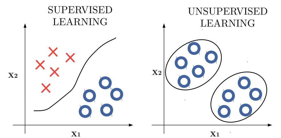
- In supervised learning, we can partition the data using a decision boundary that separates labeled classes.
- In unsupervised learning, we instead group data points according to their similarities or characteristics, without relying on predefined labels.
MOTIVATION
Most of the most impressive results in deep learning have been achieved through purely supervised learning methods (e.g., object recognition). Although progress in unsupervised learning has been slower, it is expected to play a crucial role in the future development of deep learning for several reasons:
-
Reason 1 - Data Availability
Deep learning models are typically over-parameterized, meaning they require a large amount of data to avoid overfitting. As we can imagine, it is often easier to obtain unlabeled data than labeled data, since labeling requires human intervention and can be expensive.
By leveraging unlabeled data, we can reduce the amount of labeled data needed for training, thus alleviating the overfitting problem and improving generalization.
-
Reason 2 - Discovering Hidden Structure
Frequent structures and hidden patterns are already present in data, regardless of the presence or not of a supervision signal.
Unsupervised learning involves observing multiple examples of a random vector and attempting to implicitly or explicitly learn the probability distribution , or some interesting properties of that distribution.
If I have millions of face images, there are some common patterns that emerge across all faces — for example, eyes, nose, and mouth.
Even without labels, a model can learn to represent these shared features.
-
Reason 3
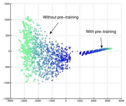
It can be highly beneficial to initialize a model not with random parameters, but with parameters pre-trained on a related domain.
In practice, we often first warm up a model using unsupervised (or self-supervised) pre-training, and then fine-tune it using supervised data.
This approach offers two main advantages:
- Optimization: to initialize parameters in a better than any position given by random initialization.
- Regularization: Unsupervised learning acts as a good regularizer for supervised learning.
Learning Representations
The MNIST dataset contains images of handwritten digits centered in a grid of pixels — theoretically allowing possible binary combinations. However, only a tiny fraction of these correspond to real digits, while the rest are meaningless or invalid configurations.
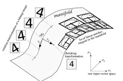
Unsupervised learning aims to discover the low-dimensional manifold where real data actually lies, reducing the vast input space to the regions that represent valid and meaningful samples.
MANIFOLD ASSUMPTION
The manifold assumption states that data lies approximately on a low-dimensional manifold embedded within the high-dimensional input space.
When this is true, it becomes more effective for machine learning algorithms to represent data using coordinates on the manifold, rather than raw coordinates in the full high-dimensional space .
FINDING A GOOD REPRESENTATION
A classic unsupervised learning task is to find the “best” representation of the data. In particular, we aim for a representation that preserves as much information about as possible, while being simpler or more structured than the original input.
The new representation can be:
- Task-specific tailored for a particular objective (e.g., recognizing a single class).
- Task-agnostic useful across multiple tasks (e.g., recognising every class)
There are three criteria for a good representation:
- Lower dimensional representations attempt to compress as much information about into a low-dimensional representations space. By forcing a model to compress input data, these techniques implicitly identify and remove redundancies while retaining the most relevant information.
- Sparse representations embed the dataset into a representation whose entries are zero for most inputs, leading to well-separated and interpretable features.
- Independent representations aim to disentangle the underlying factors of variation, making the representation dimensions statistically independent.
PRINCIPAL COMPONENT ANALYSIS
A classical example of linear dimensionality reduction is Principal Component Analysis (PCA).
PCA is an unsupervised algorithm that learns an orthogonal, linear transformation of the data—effectively finding a new set of axes. By design, the coordinates along these new axes (the principal components) are linearly uncorrelated, or “disentangled by construction”.
The goal of PCA is to preserve as much of the original data’s informative content as possible while maximizing variance along the principal components, effectively spreading the data as far apart as possible in the new subspace.
However, this linear-only approach is a significant limitation. In many real-world datasets, features have more complicated, non-linear dependencies that PCA cannot capture. To find and model these more complex structures and patterns, we must use non-linear dimensionality reduction methods.
AN INEFFICIENT WAY TO FIT PCA
One inefficient way to approximate PCA with a neural network is to use a linear autoencoder, which is a neural network with: an input layer, a “bottleneck” hidden layer (with fewer neurons, ), and an output layer with the same number of neurons as the input.
A linear autoencoder with an -neuron bottleneck, when trained to minimize squared reconstruction error, will successfully identify and span the exact same -dimensional subspace as the first principal components (PCs) from PCA.
However, the solution is not identical to PCA:
- The autoencoder’s hidden units (its “axes”) are not guaranteed to be orthogonal.
- They are not ordered by importance; instead, they tend to capture roughly equal amounts of variance from the data.
Autoencoders
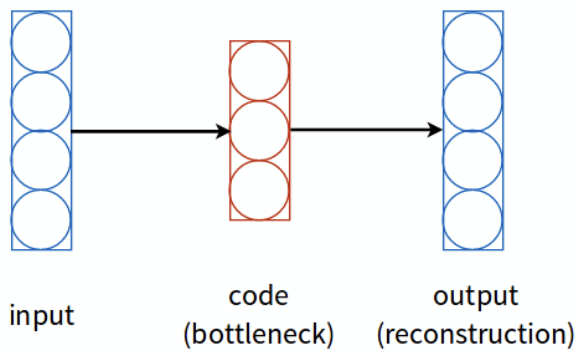
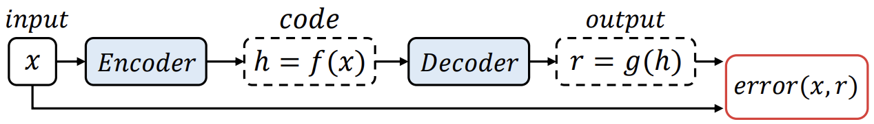
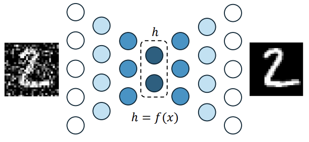
An autoencoder is a feed-forward neural network trained to copy its input to its output after performing dimensionality reduction.
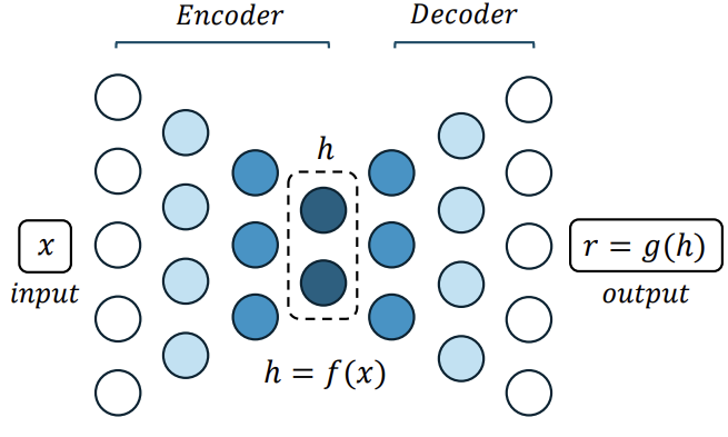
The network can be conceptually divided into two parts:
- Encoder: — maps the input to a lower-dimensional representation , often interpreted as coordinates on a manifold.
- Decoder: — reconstructs an approximation of the original input from the encoded representation.
The goal is to induce in useful properties that capture the most salient features of the training data. This representation, often called the code, has fewer dimensions than the original input.
By including nonlinear layers in both the encoder and decoder, the autoencoder can learn to represent data lying on or near a nonlinear manifold, capturing more complex structures than linear methods like PCA.
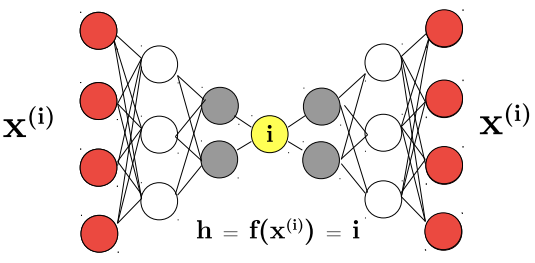
RISK: LEARN THE IDENTITY FUNCTION
An autoencoder’s goal is to learn a meaningful, low-dimensional representation (the “code”), not to simply achieve perfect reconstruction. A network that only learns to set its output equal to its input has failed its primary task.
This failure is a specific form of overfitting unique to autoencoders and unsupervised learning. In supervised learning, overfitting means memorizing the link between an input and its class. Here, overfitting means the network learns the identity function.
This problem is especially likely if the autoencoder is overparameterized or given too much capacity—for example, if the hidden code’s dimension is greater than or equal to the input dimension.
The result is that the network might achieve a perfect (zero) reconstruction loss, but the resulting code is useless. We’ve spent millions of parameters and a complex training process to learn a trivial “copy” operation,
UNDERCOMPLETE AUTOENCODER
The simplest form of autoencoder regularization is to constrain the hidden code to have a smaller dimension than the input .
This bottleneck forces the network to learn a compressed representation of the data, ideally capturing only the most salient features and variations. In this sense, an undercomplete autoencoder can be viewed as a nonlinear generalization of PCA.
The network is trained to minimize a reconstruction loss:
which penalizes the reconstruction for being dissimilar from the input — for instance, using the mean squared error (MSE).
However, simply introducing a bottleneck is not sufficient to ensure meaningful feature learning. If the encoder and decoder have excessive capacity (e.g., very deep or with many parameters), the network can still learn to perform the copying task without extracting useful information.
In this case, the decoder effectively acts as a memory bank, while the encoder learns an index to retrieve stored examples — producing perfect reconstructions for the training set but failing to generalize to new data.
Regularized Autoencoders
When training autoencoders, we face a classic trade-off:
- If the model has too few parameters, it will underfit the training set, failing to capture the relevant structure in the data.
- If the model has too many parameters, it will overfit the training set — effectively learning the identity function, and simply reproducing the input rather than learning meaningful representations.
A key principle in deep learning is to use a large model (high capacity) but constrain it with regularization.
In autoencoders, our goal is to make the latent code compact and informative. Therefore, we typically apply regularization directly to the code. This is done by adding a penalty term to the loss function that encourages the code to have desirable properties, such as sparsity, smoothness, etc.
This process creates an intelligent form of lossy compression. We accept that the reconstruction will not be a perfect copy of , because we want the network to discard irrelevant information and keep only the most salient features.
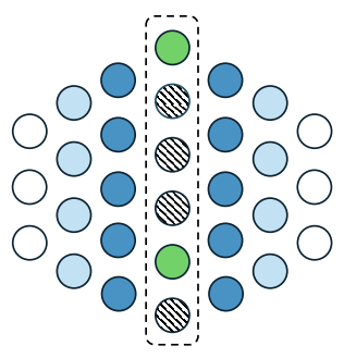
SPARSE AUTOENCODER
A sparse autoencoder is an autoencoder whose training criterion involves an additional sparsity penalty on the code layer , encouraging most of its units to remain inactive. The modified loss function is:
where:
- is typically the mean squared error (MSE) between the input and its reconstruction.
- represents the L1 norm of the code, computed as the sum of the absolute values of the activations in the hidden layer.
- (lambda) is the regularization hyperparameter that controls the trade-off between reconstruction accuracy and sparsity.
By penalizing activations in the code, the network learns a sparse representation — meaning that, for each input, only a small subset of neurons in the code layer are active. This allows the model to build an overcomplete representation (with more hidden units than inputs) without risking to learn the identity function.
Key Difference from MLP Regularization
In traditional MLPs, an L1 penalty is applied to the weights, encouraging the network to use as few connections as possible — effectively reducing model capacity.
In contrast, a sparse autoencoder applies the L1 penalty to the code activations, encouraging the latent space itself to be sparse.
This means, for example, that one neuron might activate strongly for cats, another for dogs, while the remaining neurons stay close to zero — leading to a disentangled and interpretable latent representation.
The general idea of a sparse autoencoder is to learn a “dictionary” of elementary concepts or features from the data. This dictionary is typically overcomplete, meaning its dimensionality is much higher than that of the input ().
It’s critical to understand that the model is not learning to classify or to understand the mutual relationships between objects.
If an image contains a man and a car (even if they are “messed up” in the image), the autoencoder will simply activate the “man concepts” and “car concepts” in its dictionary. Its goal is to learn a dictionary of all the concepts present in the database (e.g., “man,” “car,” “wheel,” “face”).
DENOISING AUTOENCODER
To force the hidden layer to discover more robust features, a denoising autoencoder (DAE) corrupts the input with noise (e.g., Gaussian noise) and trains the network to reconstruct the original, clean input from this noisy version. Formally, the DAE minimizes the loss:
Denoising autoencoders must therefore undo this corruption rather than simply copying their input.
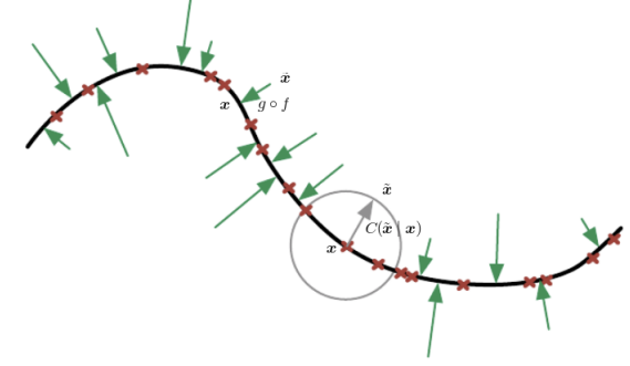
A DAE learns to project corrupted samples back onto the manifold where real, valid data lies.
In other words, the model learns a vector field that points from noisy samples toward regions of higher data probability. By knowing where each point near the curve should be projected, a DAE has implicitly learned the structure of the underlying manifold responsible for the data-generating process.
DAEs are massively used for Anomaly Detection:
-
Train the DAE with noisy versions of normal data.
-
At inference, compute the reconstruction error
-
Flag samples with high reconstruction error as potential anomalies.
CONTRACTIVE AUTOENCODER
A Contractive Autoencoder (CAE) is an autoencoder trained not only to reconstruct its input from the encoded representation, but also to make the code insensitive to small variations in the input.
This is achieved by adding a penalty term to the loss function that minimizes the gradient of the encoder activations with respect to the input:
This regularization term forces the model to learn an encoding that:
- Does not change much when changes slightly.
- Reduces the number of effective degrees of freedom in the learned representation;
- Captures only the variations necessary to reconstruct the training examples.
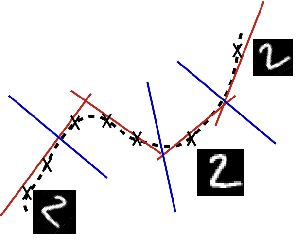
We wish to extract features that only reflect variations observed in the training set:
- The red line represents directions of variation to which the encoder must remain sensitive to reconstruct the input accurately.
- The blue line represents directions where the encoder should be insensitive, as those variations are not present in the data.
The name “contractive” comes from this behavior: the encoder is trained to resist perturbations, so it learns to map a neighborhood of input points (including those slightly off the manifold) to a smaller, “contracted” neighborhood in the code space.
By learning to be sensitive only to the “tangent planes” (the red-line directions) at each location, the CAE effectively captures the underlying structure of the data manifold.
Key Takeaways
| Concept | Description |
|---|---|
| Unsupervised learning | Groups data by similarity without labels; learns or useful properties of the distribution |
| Manifold assumption | Real data lies on a low-dimensional manifold within the high-dimensional input space |
| PCA | Linear dimensionality reduction: orthogonal axes that maximize variance; cannot capture nonlinear structure |
| Autoencoder | Neural network trained to reconstruct its input through a bottleneck: encoder , decoder |
| Identity function risk | Overparameterized autoencoders can learn to simply copy input output without extracting useful features |
| Undercomplete AE | Bottleneck with forces compression; nonlinear generalization of PCA |
| Sparse AE | Adds L1 penalty on activations: ; enables overcomplete dictionaries |
| Denoising AE (DAE) | Corrupts input with noise, trains to reconstruct clean version: ; learns the data manifold |
| DAE for anomaly detection | High reconstruction error flags anomalies — the model only reconstructs “normal” patterns well |
| Contractive AE (CAE) | Penalizes : code must be insensitive to small input perturbations |