Generative models
Variational Autoencoders
Generative modeling
Generative modeling is a class of machine learning whose goal is to learn the probability distribution of data points within a high-dimensional space . By modeling this distribution, generative models can capture the underlying structural patterns of a training dataset .
This enables them to:
- Sample new, realistic data points that resemble the original dataset.
- Support inference, that is, computing the likelihood of a data point, allowing the model to assess whether it belongs to the learned distribution. This represents a critical feature for anomaly and novelty detection.
In practical terms, such as with image data, a successful model assigns high probability to data that resembles real images and low probability to random noise.
GENERATIVE MODELING AND AUTOENCODERS
Standard autoencoders, including denoising and contractive autoencoders, are primarily discriminative, meaning they focus on learning a mapping that is useful for distinguishing between classes. Although these models can implicitly capture the structure of the data distribution by learning the geometry of the data manifold, they do not explicitly model this distribution. As a result, sampling new data points from them is difficult.
Solution: modeling the true distribution using simpler distribution that we can easily sample from.
Latent Variable Models
To model a complex distribution using a simpler one, we often map the data into a new space , known as the latent space.
The assumption is that the observed data (e.g., image pixels) are generated from unobserved variables that exist implicitly, called latent variables. These variables capture high-level factors that explain differences between data points, providing a simplified, abstract representation of the data.
Analogy: Instead of memorizing every pixel in an image of a face, the model summarizes it using key characteristics like identity, facial expression, head angle, and lighting. These characteristics act as latent variables, capturing the essential differences between images in a compact form.
The latent variables are not manually specified; the model learns them directly from the observed data to find the most efficient representation.
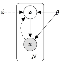
Rather than modeling directly, generative models introduce latent variables and model the joint distribution . By applying the law of total probability and the definition of conditional probability, we can express the marginal distribution of the data as:
INTRACTABILITY PROBLEM
While this provides the foundation for Variational Autoencoders (VAEs), calculating this integral is typically computationally intractable, especially in high-dimensional spaces or when the conditional distribution is complex.
To approximate this integral, a common approach is Monte Carlo estimation. Instead of calculating the full integral, we approximate it by averaging over a finite set of samples drawn from a proposal distribution (the prior) :
SAMPLING PROCEDURE
This formulation can be represented using a graphical model, where is the parent node and is the child node. The generative sampling procedure consists of:
- Sampling
- Generating from the conditional distribution
- Apply Monte Carlo approximation
VARIATIONAL INFERENCE
Using Monte Carlo methods provides some significant challenges because the quality of the approximation depends critically on the choice of latent samples. Most sampled values of are irrelevant to a specific observation ; consequently, random sampling often leads to poor estimates.
Variational Inference addresses this issue by learning a proposal distribution such that it approximates well the original . Instead of sampling blindly, the model learns a distribution that, given an observation , focuses on the most plausible latent variables —that is, those with high probability under the true posterior .
This is formulated as an optimization problem that minimizes the Kullback–Leibler (KL) divergence between the two distributions:
Minimizing this divergence ensures that the learned distribution can effectively replace the true posterior for inference. However, direct minimization is intractable because computing requires knowing the evidence , which is generally impossible for complex generative models.
DERIVING VARIATIONAL OBJECTIVE
To make the problem tractable, we start from the definition of the KL divergence:
Note: The expectation operator corresponds to an integral when the variable is continuous:
Expanding the logarithm:
By applying Bayes’ rule , we can write:
Importantly, the term does not depend on , and therefore can be moved outside the expectation:
Rearranging the terms:
Since , we obtain:
ELBO: THE EVIDENCE LOWER BOUND
By rearranging the previous equation, we obtain:
This is important because It provides a relationship between (first term of the left side) and the posterior distribution .
-
Right side
The right-hand side (the ELBO) is something we can optimize via stochastic gradient descent given the right choice of . This optimization is the core principle behind Variational Autoencoders (VAEs).
-
Left side:
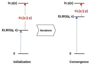
Since the KL divergence is always non-negative, the ELBO serves as a lower bound on the true log-likelihood:
Why Maximizing the ELBO Works?
Maximizing the ELBO is equivalent to minimizing the KL divergence between the approximate posterior and the true posterior .
This is because the depends only on the data and the model parameters — it is constant with respect to the variational distribution . Therefore, as we push the ELBO “up” toward , the “gap” (the KL divergence) must necessarily shrink.
Variational Autoencoder (VAE)
A Variational Autoencoder (VAE) is an autoencoder trained to maximize the Evidence Lower Bound (ELBO):
where:
- Reconstruction term, encourages accurate reconstruction of the input data,
- Regularization term, forces the approximate posterior to remain close to a chosen prior distribution , which is typically a Gaussian distribution.
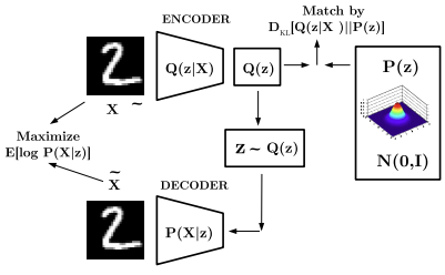
ARCHITECTURE
The VAE architecture maintains the encoder–decoder structure of standard autoencoders. However, instead of mapping the input to a single deterministic latent vector, the encoder outputs the parameters — typically the mean and variance — of a latent distribution.
Components:
- Encoder network : Given an input , the encoder estimates the posterior distribution over latent variables. In practice, this is usually modeled as a multivariate Gaussian: such that . The network outputs two vectors, and , representing the parameters of the approximate posterior.
In practice, the encoder projects the data into the space of latent variables.
-
Decoder network : The decoder reconstructs the input data from a latent sample . A latent vector is drawn from the approximate posterior and the decoder produce a reconstruction that aims to match the original input :
In practice, the decoder network learns the conditional distribution and tries to reconstruct the input as accurately as possible.
To maximize the log-likelihood , the model typically minimizes the Mean Squared Error (MSE) between input and reconstruction.
REGULARIZATION
The Regularization term in the ELBO objective is defined as:
This term measures how much the approximate posterior produced by the encoder diverges from the prior distribution .
The prior represents our prior belief about the distribution of the latent variables before observing any data. It is typically “hand-crafted” as a Standard Multivariate Gaussian:
Why use a Gaussian Prior? Choosing a Gaussian distribution for is a standard practice in VAEs for several reasons:
- Computational Efficiency: If both the approximate posterior and the prior are Gaussian, the KL divergence has a closed-form solution. This allows it to be computed exactly using a fixed formula, without numerical approximation or sampling, making training efficient.
- Well-Behaved Latent Space: A standard Gaussian encourages the latent space to be centered, compact, smooth, and connected, preventing the model from spreading latent codes infinitely apart.
- Simplicity: A Gaussian prior provides a simple, data-independent reference distribution, allowing the model to learn complex data structure through the encoder rather than through the prior.
REPARAMETRIZATION TRICK
A critical implementation challenge in VAEs arises from the sampling operation:
Sampling is stochastic and therefore non-differentiable, which prevents gradients from flowing through the latent layer to the encoder.
To address this problem, we use the reparameterization trick. Instead of sampling directly from the approximate posterior:
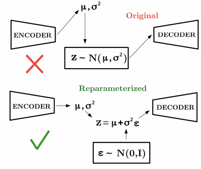
- Sample Noise: Draw from a standard normal distribution of the same dimension as :
- Reparametrize: We then compute using the parameters provided by the encoder:
This transformation produces a sample that is statistically equivalent to sampling from the original distribution , but now gradients can flow through and during backpropagation.
Advantages:
- The stochasticity is isolated in , whose distribution does not depend on the encoder parameters, allowing standard gradient-based optimization to train the model efficiently.
SAMPLING IMAGES AFTER TRAINING
Once a Variational Autoencoder has been successfully trained, the learned posterior closely matches the prior . This allows new data points to be generated by sampling directly from the prior.
A sampled latent vector is then fed into the decoder, which transforms it into a generated image. This process works because, during training, the decoder has learned to reconstruct inputs from latent variables that were explicitly encouraged to follow the prior distribution. As a result, any latent sample drawn from can be decoded into a realistic new data point, enabling the VAE to generate entirely novel images that resemble the training data.
Generative Adversarial Networks
WHY GANs?
Generative Adversarial Networks (GANs) were introduced to address limitations of likelihood-based generative models such as VAEs.
Limitations of VAEs / VQ-VAEs
VAEs often generate blurry images mainly because:
- Likelihood-based training (MSE ): The VAE decoder is typically trained by minimizing pixel-wise MSE. If the model is uncertain about the exact position of details, it averages the possibilities, resulting in a blurry line.
- Strong regularization (KL term): The latent posterior is forced to match a simple prior (e.g., standard normal). If this regularization is too strong, the latent representation may lose important information (posterior collapse).
GANs: A Different Approach
Unlike VAEs, GANs do not require an explicit density function. Instead of modeling the data distribution directly, they learn a generator that maps noise directly to real data distribution via adversarial training.
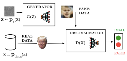
ADVERSARIAL TRAINING NETWORKS: ARCHITECTURE
Generative Adversarial Networks (GANs) are another generative approach, based on two networks that compete with each other, in a game theoretic scenario:
-
The generator network
The generator’s goal is to produce realistic samples that can “fool” the discriminator. During training, its objective is to maximize the probability of the discriminator making a mistake. In order to do so:
- It takes random noise from a simple distribution (e.g., Uniform or Gaussian).
- Transform this noise into a data sample in the target domain (such as an image).
-
The discriminator network
The discriminator acts as a binary classifier that evaluates the authenticity of the data. It receives samples from both the training set and the generator, then it emits a probability value indicating whether the input image is “real” (from the data distribution) or “fake” (from the generator).
LOSS
The Generator () and Discriminator () are trained jointly using a Minimax Objective Function:
- The Discriminator () wants to maximize the objective such that is close to 1 (real) and is close to 0 (fake):
-
The first term is the expectation over real data samples :
Maximizing this term encourages the discriminator to assign high probability to real data.
-
The second term is the expectation over generated samples :
Maximizing this term encourages the discriminator to assign low probability to generated (fake) samples.
-
is trained to maximize its classification accuracy across both real and synthetic datasets.
-
The Generator () aims to minimize the objective such that is close to 1 as possible (effectively “fooling” the discriminator).
Since the generator only appears in the second term, it seeks to minimize . Like that it is forced to produce increasingly realistic samples.
TRAINING DYNAMICS The two optimizers operate on separate sets of parameters, even though the overall loss depends on both. Training typically alternates between two steps:
- Gradient ascent on discriminator:
Updating the Discriminator to improve its classification.
-
Gradient descent on generator:
Updating the Generator to produce samples that better evade the discriminator’s detection.
Convergence is reached when the generator produces data indistinguishable from real data, and the discriminator cannot reliably differentiate between the two.
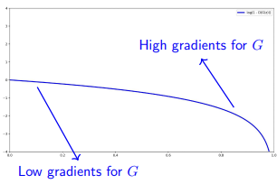
TRAINING GANs: VANISHING GRADIENTS PROBLEM
Problem: If the discriminator is too good and the generator is not yet producing realistic samples, the generator will receive very small gradients, leading to vanishing gradients.
In the original GAN formulation, the generator minimizes:
If the discriminator correctly classifies fake samples, then:
- is close to 0
- is close to 0,
and the gradient of this term becomes very small. As a result the generator fails to learn because it receives almost no useful feedback to update its parameters.
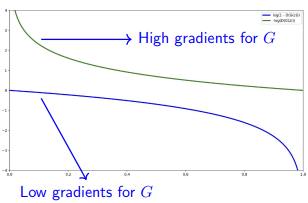
Solution: To address this, we modify the generator’s objective. Instead of minimizing the probability of the discriminator being correct, we maximize the probability of the discriminator being wrong.
We switch the generator’s objective to:
This alternative formulation provides stronger gradients even when the discriminator performs well, improving training stability:
By receiving stronger feedback in the early stages of training, the generator can more quickly learn to produce samples that resemble the real data distribution.
TRAINING ALGORITHM
Algorithm 1 Minibatch stochastic gradient descent training of generative adversarial nets. The number of steps to apply to the discriminator, , is a hyperparameter.
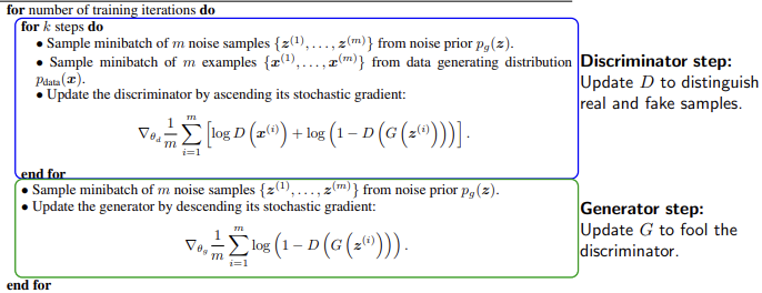
It is common to perform multiple discriminator updates per generator update (e.g., discriminator steps and 1 generator step).
PROS AND CONS
- Pros:
- Can utilize power of backpropagation
- The loss function is learned instead of being hand selected
- No MCMC needed
- Cons:
- Trickier and more unstable to train
- Need to manually babysit during training
- No evaluation metric, so it’s hard to compare with other models
Deep Convolutional GANs
Adversarial training is inherently unstable as it requires maintaining a delicate balance between two competing networks. DCGANs were the first architecture to replace fully connected layers with Convolutional Neural Networks (CNNs) in both the generator and discriminator. This significantly improved image quality and training stability.
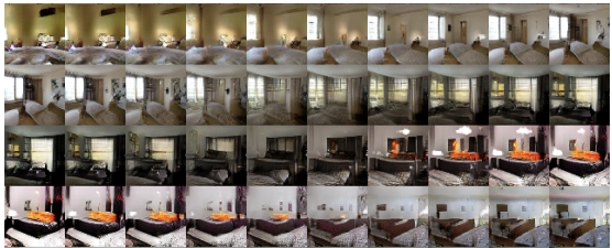
A key property of DCGANs is the smooth interpolation in the latent space: moving between random latent vectors produces gradual and realistic transitions in the generated output.
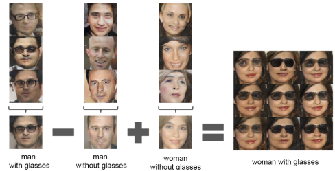
SEMANTIC LATENT SPACE ARITHMETIC
Latent vectors in DCGANs exhibit semantic properties. Moving along specific directions in the latent space corresponds to meaningful transformations, such as changing a subject’s gender, adding glasses, or modifying facial attributes (e.g., “Man with glasses” - “Man” + “Woman” = “Woman with glasses”).
IMPROVING STABILITY: LSGAN AND WGAN
To prevent one network from dominating the other and to mitigate gradient saturation, alternative loss functions were proposed:
- Least Squares GAN (LSGAN) Replaces the binary cross-entropy loss with a least squares objective, which provides a smoother gradient and penalizes samples that are far from the decision boundary.
- Wasserstein GAN (WGAN): Uses the Wasserstein distance (Earth Mover’s distance) instead of the original Jensen-Shannon divergence. This provides more stable gradients and requires enforcing Lipschitz continuity (often via weight clipping or gradient penalty).
SPECIALIZED ARCHITECTURES
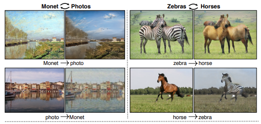
CycleGAN: unpaired image-to-image translation
CycleGAN is designed for domains where paired training data (e.g., the exact same photo in “summer” and “winter” versions) is unavailable. It employs two generators (, ) and two discriminators.
The core principle is Cycle Consistency:
This ensures that an image translated from domain A to B and back to A reconstructs the original input, preventing the model from losing the structural content of the image.
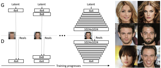
Progressive GAN
This architecture starts by training on very low-resolution images (e.g., 4x4) and progressively adds layers to both the generator and discriminator to handle higher resolutions. This approach is essential for generating very high-resolution outputs (e.g. 1024x1024).
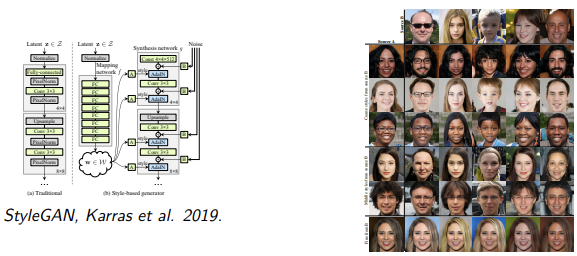
StyleGANs
StyleGAN introduces a generator architecture based on “style” to allow fine-grained control over image attributes.
Instead of using the latent vector directly, it is transformed into a style vector via an MLP. This disentangles the latent space, ensuring that similar vectors don’t overwrite unrelated features.
The style vector is translated into scale () and bias () parameters that normalize the feature maps:
Uncorrelated Gaussian noise is added to each convolutional layer to generate fine details like pores, hair follicles, or freckles without affecting the global structure.
Key Takeaways
| Concept | Description |
|---|---|
| Generative modeling | Learn to sample new data and assess likelihood; enables anomaly detection |
| Latent variable models | Model ; latent variables capture high-level factors of variation |
| Variational inference | Learn a proposal by minimizing KL divergence; avoids blind Monte Carlo sampling |
| ELBO | ; tractable lower bound on |
| VAE | Encoder outputs of a Gaussian posterior; decoder reconstructs from sampled ; trained via ELBO |
| Reparameterization trick | , ; makes sampling differentiable for backpropagation |
| GAN | Generator vs. discriminator ; minimax game — no explicit density needed |
| GAN vanishing gradients | When is too strong, gets near-zero gradients; fix: maximize instead of minimizing |
| DCGAN | CNNs in both and ; smooth latent interpolation and semantic arithmetic in latent space |
| CycleGAN | Unpaired image-to-image translation via cycle consistency: |
| Progressive GAN | Trains from low-res to high-res by progressively adding layers; enables 1024x1024 generation |
| StyleGAN | Maps via MLP for disentangled control; AdaIN injects style; noise adds fine details |