Self-Supervised Learning
Introduction
In traditional supervised learning, models rely on labeled data, but high-quality labeled datasets are often limited, expensive, or unavailable. In many real-world applications, such as industrial anomaly detection, historical examples of specific events (like equipment failures) are rare and costly to document. Other domains may require significant human expertise and labor for manual annotation.
Self-supervised learning addresses these limitations by automatically generating supervision signals from the data itself. This specific form of representation learning enables models to learn useful representations of the data from unlabeled datasets.
Learning good representations makes easier the transfer of information to downstream tasks, such as:
- Tasks with only a few available examples
- Zero-shot transfer to new tasks.
The approach is motivated by the idea of constructing supervised learning problems directly from unlabeled data.
TAXONOMY
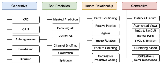
SELF-SUPERVISED LEARNING VS GENERATIVE LEARNING
A key distinction between these two approaches lies in the level of detail required for the learning objective:
- Generative Models: aim to reconstruct all details of the data, focusing on high-fidelity reproduction.
- Self-Supervised Methods: focus on predicting higher-level semantic features or abstract properties through pretext tasks.
The ultimate goal of SSL is to capture the general context and the most important features of the data to develop robust representations, rather than reconstructing every pixel.
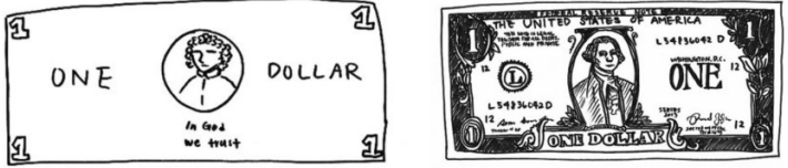
Left: Drawing of a dollar bill from memory. Right: Drawing subsequently made with a dollar bill present
PRETEXT TASK
A pretext task is a synthetic prediction problem derived directly from the data. Its primary purpose is to force the model to learn useful features by generating labels automatically, without human intervention.
EXAMPLE: PREDICTING THE ROTATION ANGLE
A classic pretext task is rotation prediction, where the model is trained to identify the orientation of an image:
- Input: An image is rotated by a specific angle (e.g. 0°, 90°, 180°, or 270°)
- Objective: Predict which of the four rotations was applied
It turns out to be a simple 4-way classification task.
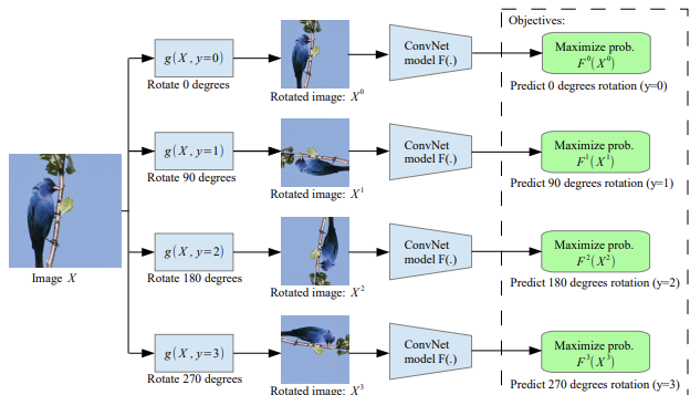
Solving it requires the model to understand the structure of objects in the image. The model is not learning how to rotate the image; instead, it learns general concepts, such as the typical location of a bird’s head, wings, and body, and how objects usually appear in a canonical orientation. This forces the network to capture meaningful visual features and spatial relationships.
The pretext task is used only to extract useful features, which can then be transferred to real downstream tasks.
EVALUATION OF A SSL METHOD
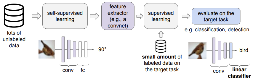
Self-supervised learning is typically used in a two-stage pipeline:
-
Pretraining phase
The model is trained on a vast amount of unlabeled data using a pretext task (e.g., predicting image rotations). The goal is to develop a robust feature extractor that captures meaningful patterns and structures without human-provided labels.
-
Fine-Tuning phase
After pretraining, the learned feature extractor is adapted to a downstream task (e.g., classification or detection). A shallow network (often just a few linear layers) is attached to the pretrained feature extractor and trained on a small set of labeled data for the target task. Since the model already understands fundamental features from the pretraining phase, it requires significantly fewer labeled samples to reach high performance.
This approach leverages the strengths of both large-scale unlabeled data and supervised learning. It is sometimes referred to as semi-supervised learning, as it combines unlabeled pretraining with labeled adaptation.
Why predicting rotations?

A model that can correctly predict the rotation of an input image also learns strong visual features, as it develops a form of “visual commonsense” about how objects should appear in their normal, unrotated orientation.
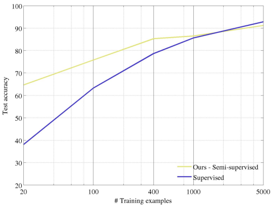
As we can see models pretrained with self-supervised tasks require fewer labeled examples to achieve high accuracy on downstream tasks.
As the number of labeled examples grows (e.g., 100 or 400 per class), the advantage of self-supervised pretraining decreases, since sufficient labeled data alone can achieve high performance.
This shows that self-supervised learning is most valuable in low-data regimes, while direct supervised training may be sufficient when large labeled datasets are available.
SSL through intra-example relationships
Self-supervised learning often leverages spatial transformations to force a model to understand object composition and context without manual labels.
Pretext Task: Jigsaw Puzzles
PERMUTATION PREDICTION
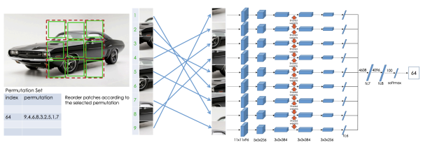
In this self-supervised task, a model is trained by dividing an image into patches so that it can learn how the patches are spatially arranged. The goal is to develop high-level structural representations of objects rather than pixel-level reconstructions.
The training procedure is the following:
- Define Permutations: A finite set of valid patch permutations is predefined.
- Apply Shuffling: Each image is divided into patches and shuffled according to one of the predefined permutations to generate training samples.
- Processing: Every patch is processed by the same neural network using shared weights.
- Joint Observation: The resulting embeddings are concatenated, allowing the model to consider all tiles simultaneously and learn the relationships between them. This joint observation removes ambiguity because patch placements are mutually exclusive.
- Predict: The model outputs a probability vector to classify which specific permutation was used.
To succeed, the model must acquire two levels of understanding:
- Patch-level Semantics: Recognizing the identity of individual components in an object, such as distinguishing the eye from a background.
- Spatial Relationships: Learning where these parts typically appear relative to one another.
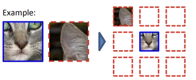
RELATIVE PATCH POSITIONING
A related variant involves extracting random pairs of patches from an unlabeled collection to predict their spatial relationship.
Instead of predicting the full permutation:
- Two patches are sampled from the same image.
- One patch is treated as a reference.
- The model predicts which of the eight neighboring positions (top, bottom, left, right, or the four diagonals) the second patch occupies relative to the first..
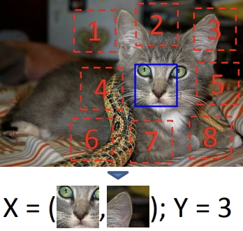
This method emphasizes the interactions between parts over their individual identities. Success in this task demonstrates that the model has learned to recognize objects and the logical arrangement of their components.
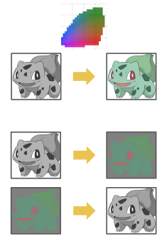
Pretext Tasks: Colorization
Image colorization is a self-supervised learning technique where a model is given a grayscale image as input and trained to reconstruct plausible colors.
The primary goal is not the color reconstruction itself, but the robust representations learned during the process. To colorize an image accurately, the model must acquire a form of visual common sense by learning:
- Semantic Recognition: Identifying objects such as sky, water, vegetation, and buildings.
- Color Coherence: Maintaining consistent color across neighboring pixel
- Regularities and Constraints: understanding that certain objects tend to have typical colors, while others are implausible (e.g., sky is usually blue, vegetation green, roads gray). In this way, color becomes a proxy for object recognition.
TECHNICAL VARIATIONS
- CIE Lab Color Space: Specifically, the task often involves predicting binned colors from the CIE Lab color space based on a grayscale input.
- Split-brain Autoencoder: A generalization of colorization that predicts a subset of color channels (such as color or depth) from the remaining channels, such as luminosity.
APPLICATIONS BEYOND FEATURE LEARNING
Since these models are trained on artificially generated grayscale images, they can be applied to real black-and-white photographs to produce realistic colorized versions, for example in satellite imagery.
Self-prediction
Self-prediction is a family of self-supervised methods based on reconstruction tasks. The core concept is to hide a specific portion of an individual data sample and train the model to reconstruct it using the remaining visible parts. This approach can be applied to various data types, including images, sequences, and time series.
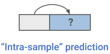
In these tasks, the part to be predicted is treated as if it were missing. By pretending the model does not have access to that information, the model is forced to learn the underlying structure and relationships within the data.
Self-prediction: given an individual data sample, the task is to predict one part of the sample given the other part.
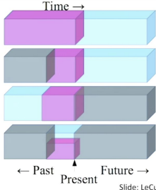
Common self-prediction tasks include:
- Temporal Prediction: Predicting the future from the past or the recent past, or even predicting the past from the present.
- Spatial Prediction: Predicting the top half of an image from the bottom half, or reconstructing occluded regions from visible ones.
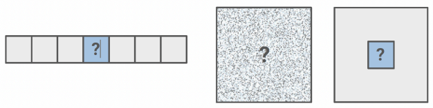
Self-prediction generally falls into three main categories based on the generation strategy:
- Masked Generation: Predicting randomly hidden or “masked” parts of the input.
- Autoregressive Generation: Predicting the next element in a sequence based on all preceding elements.
- Hybrid Self-Prediction: Combining different prediction strategies within the same framework.
MASKED GENERATION
The core concept of masked generation is to hide a random portion of data, pretend it is missing and train the model to predict the missing information given other unmasked information.
Key Examples:
- Language: Masked Language Modeling, such as BERT.
- Images: masked patch (Inpainting, Masked Auto-Encoder)
INPAINTING
Inpainting consists in generating the contents of an arbitrary image region conditioned on its surroundings. So, learning to inpaint by reconstruction means learning to reconstruct the missing pixels.
To succeed at image reconstruction (inpainting), the model must understand the global content of the image and produce a plausible hypothesis for the missing parts. This process forces the network to learn:
- Visual Semantics: Capturing the meaning of visual structures rather than just surface appearance.
- Contextual Dependencies: Learning spatial relationships and object continuity.
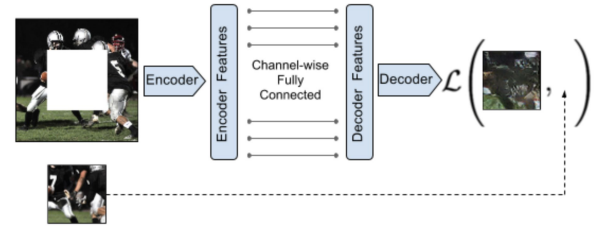
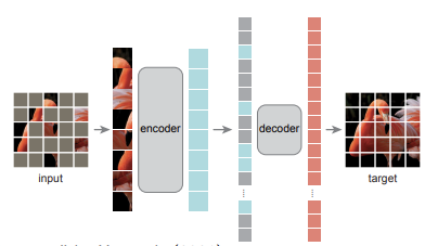
MASKED AUTO-ENCODER — MAE
Masked Auto-Encoders (MAEs) mask random patches from the input image and reconstructs the missing patches in the pixel space.
Design and Training
- High Masking Ratio: A large fraction of the image patches (often 80–90%) is removed.
- Asymmetric Encoder-Decoder:
- Encoder: Operates only on the visible patches (without mask tokens) to produce embeddings.
- Decoder: Receives the latent representations plus mask tokens representing the missing patches to reconstruct the original input.
- Selective Loss: The loss function is computed only on the masked patches, forcing the model to infer missing content from the available context.
After training, the decoder is discarded, and the encoder acts as a powerful feature extractor for downstream tasks. This design is computationally efficient because the encoder processes only the visible patches, reducing memory and computation costs.
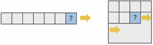
AUTOREGRESSIVE GENERATION
Autoregressive models predict future behavior based on past behavior. Any data with an inherent sequential order can be modeled in this way.
A common example is next-token prediction, where the model predicts the next word in a sequence given the preceding words. This requires no manual labels and allows the model to learn grammar, syntax, and semantic structure from raw data.
Examples:
- Audio (WaveNet, WaveRNN)
- Autoregressive language modeling (GPT, XLNet)
- Images in raster scan (PixelCNN, PixelRNN, iGPT)
Contrastive Learning
PRETEXT TASKS: ADVANTAGES AND DISADVANTAGES
The effectiveness of self-supervised learning depends heavily on the design of the pretext task. While these tasks are powerful for feature extraction, they come with specific trade-offs.
Pros
- Visual Common Sense: Pretext tasks like rotation prediction, inpainting, patch rearrangement, and colorization force the model to acquire “visual common sense”.
- Feature Quality: To solve these tasks, models must learn high-level features of natural images.
- Downstream Utility: We don’t care about the performance of these pretext tasks but rather how useful the learned features are for downstream tasks (classification, detection, segmentation).
Cons
- Problem 1: Identifying individual pretext tasks is a tedious and manual process.
- Problem 2: The learned representations may not always generalize well across different domains.
- Problem 3: Learned representations may be tied to a specific pretext task.
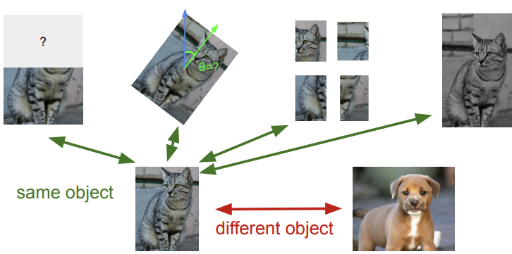
A MORE GENERAL SSL TASK: CONTRASTIVE REPRESENTATION LEARNING
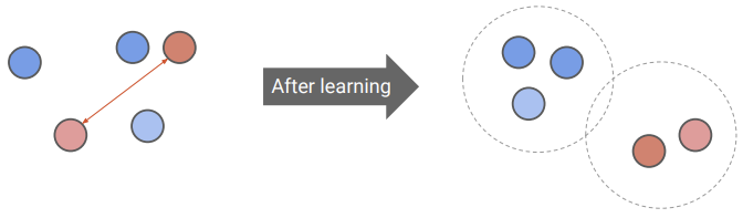
Contrastive learning is a more general self-supervised approach that moves away from specific pretext tasks. Instead of predicting a specific transformation (like a rotation angle), the model learns an embedding space by comparing different data samples.
The goal of contrastive representation learning is to map data into a space where:
- Positive pairs are pulled together: different augmented versions of the same input (e.g., cropped or color-shifted views of the same image) are mapped close to one another
- Negative pairs are pushed apart: representations of different inputs are placed far from each other
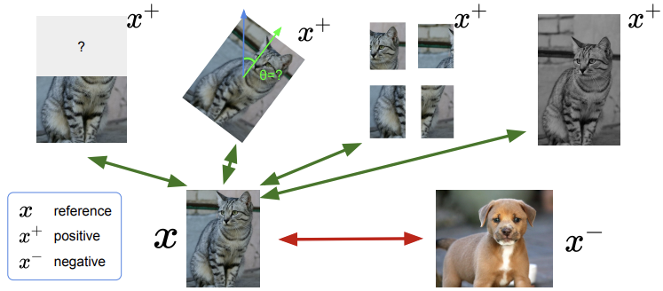
The mathematical objective of contrastive learning is to optimize an encoder function such that:
- (Anchor): The reference data sample.
- (Positive sample): A sample semantically related to the anchor.
- (Negative sample): A sample unrelated to the anchor.
The encoder must yield a high similarity score for positive pairs and a low score for negative pairs .
POSITIVE MINING STRATEGIES
Constructing the set of positive pairs is a critical step in self-supervised learning. Common strategies include:
- Data Augmentation: Pairing the original input with a distorted version of itself (e.g., through cropping, rotating, etc.).
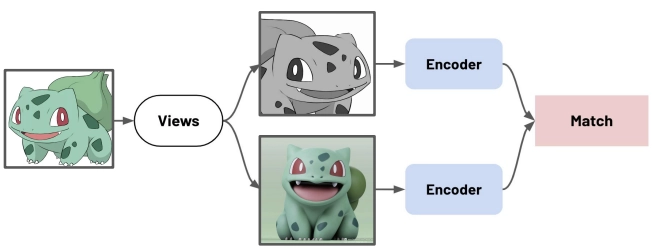
- Multi-view Learning: Using data that captures the same target from different views
Common Loss Functions
Some examples of Loss functions:
- Contrastive loss (Chopra et al. 2005)
- Triplet loss (Schroff et al. 2015; FaceNet)
- Lifted structured loss (Song et al. 2015)
- Multi-class n-pair loss (Sohn 2016)
- Noise contrastive estimation (“NCE”; Gutmann & Hyvarinen 2010)
- InfoNCE (van den Oord, et al. 2018)
- Soft-nearest neighbors loss (Salakhutdinov & Hinton 2007, Frosst et al. 2019)
CONTRASTIVE LOSS
Contrastive loss works with labelled dataset and ensures samples from the same class have similar embeddings, while samples from different classes have different ones.
For a pair of data points , the loss is defined as:
- Positive Pairs: The loss minimizes the Euclidean distance between their embeddings.
- Negative Pairs: The loss penalizes distances that are smaller than a predefined margin .
The role of the Margin
The margin serves as a tolerance threshold for separating dissimilar samples. Once two samples from different classes are separated by at least this distance (), the loss becomes zero and they are no longer penalized.
By enforcing a minimum separation, the margin prevents:
- Collapsed solutions where all embeddings become too similar.
- Over-optimization by ignoring negative pairs that are already sufficiently distant
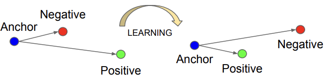
TRIPLET LOSS
Triplet loss is a training objective that simultaneously optimizes the relationships between three different samples: an anchor (), a positive (), and a negative ().
The objective is to ensure that the distance between the anchor and the positive sample is smaller than the distance between the anchor and the negative sample by at least a specified margin :
So given a triplet input , the model minimizes the following loss function:
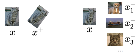
InfoNCE
InfoNCE (Information Noise Contrastive Estimation) uses categorical cross-entropy loss to identify a single positive sample from a set of unrelated negative “noise” samples.
Given an anchor , one positive sample , negative samples and a similarity function , the loss is defined as:
This loss is essentially a standard cross-entropy loss for an -way softmax classifier. The model is trained to correctly classify the positive sample out of total candidates.
The loss applies a softmax-like normalization to transform similarity scores into a probability distribution.
SIMCLR: A SIMPLE FRAMEWORK
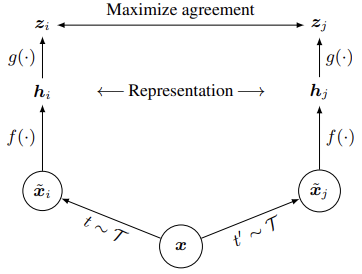
SimCLR (Simple Framework for Contrastive Learning) is a self-supervised framework that learns representations by maximizing agreement between differently augmented views of the same example thanks to a contrastive loss in the latent space.
The pipeline
Starting with a single image , the framework follows these steps:
- Data Augmentation: Two different augmentation operators ( and ) are sampled from the same family and are applied to produce two correlated views, and , forming a positive pair.
- Base Encoder : A neural network extracts feature representations () from the augmented inputs.
- Projection Head : A small neural network (typically a MLP) maps the representations into a space where the contrastive loss is applied.
Applying the contrastive loss in the projection space rather than the representation space allows the model to preserve more information in . After training, is discarded, and only the encoder is used for downstream tasks.
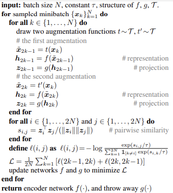
SimCLR does not explicitly sample negative examples. Instead, for a minibatch of images, it generates augmented views. For any given positive pair, the other augmented examples in the batch are treated as negatives. Thus, the batch itself provides supervision without requiring labels.
Loss Function
The model is trained using the InfoNCE loss to maximize the similarity of positive pairs and minimize the similarity of negative pairs. For a positive pair , the loss is defined as:
where:
-
denotes a temperature parameter that scales the input.
-
Similarity Metric: cosine similarity is used:
SimCLR’s Pseudocode
TRAINING LINEAR CLASSIFIER ON SIMCLR FEATURES
- Encoder Pretraining: The feature encoder is trained on a large-scale unlabeled dataset, such as the entire ImageNet training set, using the SimCLR framework.
- Linear Evaluation: The feature encoder is then frozen, and a linear classifier is trained on top of it using labeled data.
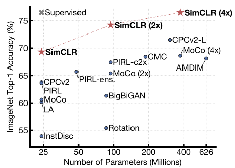
DESIGN CHOICES: LARGE BATCH SIZE
A defining characteristic of SimCLR is the use of very large training batch sizes to achieve strong performance. This is because a large number of negatives provides stronger supervision for the contrastive loss without requiring labels.
However, this choice has computational implications:
- Memory footprint: Large batches substantially increase memory usage during backpropagation.
- Hardware requirements: Training on datasets such as ImageNet often requires distributed setups on specialized hardware (e.g., TPUs) due to these memory and computational demands.
These trade-offs motivate alternative contrastive methods (such as MoCo and BYOL) that decouple the number of negatives from the batch size, achieving comparable performance with significantly lower hardware requirements.
Key Takeaways
| Concept | Description |
|---|---|
| Self-supervised learning (SSL) | Generates supervision signals from the data itself; learns representations from unlabeled data for downstream tasks |
| Pretext task | Synthetic prediction problem (rotation, jigsaw, colorization) that forces the model to learn useful features without labels |
| Two-stage pipeline | Pretrain on unlabeled data with a pretext task, then fine-tune on a small labeled dataset for the target task |
| Jigsaw puzzles | Predict spatial arrangement of shuffled image patches; learns patch-level semantics and spatial relationships |
| Colorization | Predict colors from grayscale; forces the model to learn semantic recognition and object-color associations |
| Self-prediction | Mask or hide part of the input, predict it from the rest; includes masked generation and autoregressive generation |
| Masked Auto-Encoder (MAE) | Masks 80-90% of image patches; encoder processes only visible patches, decoder reconstructs masked ones |
| Contrastive learning | Pull positive pairs (augmented views of same input) together, push negative pairs apart in embedding space |
| InfoNCE loss | Cross-entropy over -way softmax: identify the positive sample among negatives |
| SimCLR | Contrastive framework: augment encode project InfoNCE loss; uses large batches as implicit negatives |
| Projection head | MLP maps representations to contrastive loss space; discarded after training to preserve richer features in |