Continual Learning
Introduction
HUMANS AND MEMORIES
Human beings can learn new tasks while still remembering what they learned earlier. Even after focusing on a long sequence of activities, we retain past knowledge and can recall and apply it when needed.
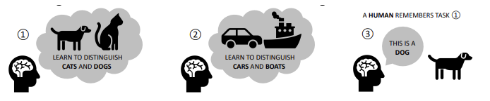
In contrast, Neural Networks trained on a continuously changing stream of data tend to forget previously learned tasks as they focus on new examples.
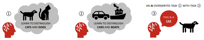
Example: if a model is first trained to classify cats and dogs, and then it is retrained on a new task — such as distinguishing cars from boats — it will typically forget how to recognize cats and dogs.
As a result, the network becomes biased toward the most recently learned classes, losing its earlier generalization capabilities.
DYNAMICS OF FORGETTING
Consider the following two tasks:
- Task 1: participants memorize a set of word pairs (e.g., home–star, field–sky, …).
- Task 2: the right-hand items of the pairs are changed (e.g., home–field, field–car, …)
As humans are exposed to more pairs from Task 2, it is natural that they forget part of what they learned in Task 1.
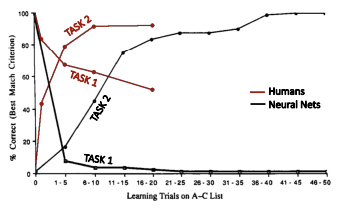
However, when the same experiment is performed with Artificial Neural Networks, the degradation is far more dramatic: just a few training steps on the new pairs are enough to drive the accuracy on Task 1 close to zero.
This phenomenon is an intrinsic property of standard neural networks, and it is known as Catastrophic Forgetting.
CATASTROPHIC FORGETTING: WHY?
Neural Networks forget mainly because of the optimization algorithm, typically based on gradient descent or one of its stochastic variants (e.g., SGD).
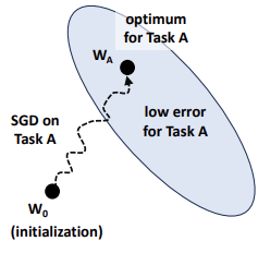
A neural network is defined by a set of parameters (weights and biases). Training on the first task starts from some initial point in parameter space and converges to a local minimum , located in a region where the loss for Task A is low.
Now consider a second task (Task B), which has its own loss landscape, completely independent of the loss for Task A. To learn Task B, the network must update its parameters. Since SGD optimizes only the current objective, it freely moves through the parameter space toward a new local minimum , without taking into account the performance on Task A.
As a consequence:
- Loss for Task B → low 🙂
- Loss for Task A → high 🙁
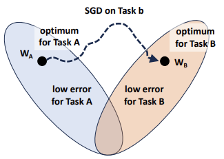
All guarantees obtained for Task A are effectively overwritten. This behavior leads directly to catastrophic forgetting.
Theoretically, NNs are over-parametrized. This means that, in theory, there should exist a set of parameters that performs well on both tasks and lies not far from the original solution .
The goal of continual learning is therefore to guide optimization toward this shared region — where both losses are low — instead of greedily minimizing only the new task loss.
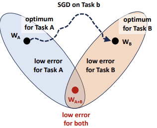
To do this, we must modify the behavior of gradient descent, adding constraints or regularization terms that preserve important knowledge from previous tasks.
Continual Learning
Continual Learning (CL) focuses on training machine learning systems on a continuous stream of changing data. The goal is to acquire new knowledge while avoiding catastrophic forgetting and without retraining the entire system from scratch whenever new data arrives.
Naïve approach
A simple solution would be to concatenate the training sets of Task A and Task B and train the model jointly. With joint training, catastrophic forgetting does not occur because the model is trained on all tasks simultaneously.
However, this approach is impractical: storing all past data is inefficient, and in many scenarios training can only be performed on the new incoming data.
To address this, CL techniques constrain how a network learns new tasks to preserve performance on old ones. For instance, parameter updates can be restricted to remain within regions that keep the loss for Task A low.
Since data from Task A is unavailable during Task B, the model must identify and protect the specific parameters critical to its previous knowledge while learning exclusively from new examples.
MATHEMATICAL FORMULATION
In a CL classification problem, training is split into sequential tasks. During each task , input samples and ground truth labels are drawn from an i.i.d. distribution .
The objective is to learn a model that performs well on all tasks, by optimizing a function with parameters sequentially. At the current task , the model must correctly classify examples from all tasks observed so far. This is achieved by minimizing the cumulative loss:
where:
- is the loss function (e.g., cross-entropy for classification), which measures how far the model’s prediction is from the ground truth. Lower loss values correspond to better predictions.
- denotes the expected value (average) of the loss over the data distribution of task .
The main challenge is to find the parameter configuration that minimizes the cumulative loss without access to the original datasets of previous tasks ().
Elastic Weight Consolidation
Elastic Weight Consolidation (EWC) is one of the earliest and most influential methods proposed to mitigate catastrophic forgetting. It is inspired by two key biological mechanisms:
- Plasticity: The ability of neural connections to modify their activity in response to stimuli.
- Synaptic Consolidation: The process where the brain stabilizes synapses critical to learned tasks, reducing their plasticity over time to protect established knowledge, while allowing new information to be encoded in less critical areas.
In continual learning
In the context of CL, the plasticity of a weight determines how much it can be modified when learning a new task:
- Low Plasticity: If a weight was important for Task A, it should remain close to its previous value.
- High Plasticity: If a weight was not important, it can be modified more freely during Task B.
EWC implements synaptic consolidation by using a quadratic regularization term to constrain important parameters to their old values.
LOSS FUNCTION
To learn Task B while staying in a parameter region where Task A still performs well, the total loss function is defined as:
Where:
- is the standard loss for Task B (e.g., cross-entropy for classification).
- is the set of optimal parameters learned for Task A.
- is the Fisher Information Matrix, which estimates the importance of parameter for Task A:
- A large forces the parameter to stay near .
- A small allows the parameter to deviate more.
- is a hyperparameter controlling the strength of the regularization.
The regularizer acts like an elastic spring, anchoring important parameters to their previously learned values—hence the name Elastic Weight Consolidation.
HOW TO ESTIMATE PER-PARAMETER IMPORTANCE?
EWC determines parameter importance using the diagonal of the empirical Fisher Information Matrix, calculated at the optimum of the first task (). For Task A, the Fisher Information is computed as:
By multiplying the gradient by its transpose, we obtain a matrix that captures the influence of every pair of parameters. EWC focuses specifically on the diagonal, which contains the importance indicators for individual weights. This simplifies the calculation to a per-parameter estimate:
Consequently, a simple moving average of squared gradients provides a practical approximation of the importance of each parameter.
Why squared gradients?
Taking the square removes any dependence on the sign → we care about the magnitude of influence, not the direction.
FISHER INFORMATION MATRIX
The empirical Fisher Information Matrix (FIM) has a strong theoretical relationship with the second derivative of the loss function. It essentially measures the curvature of the log-likelihood function around a minimum:
-
High Curvature (High Fisher Information):
The log-likelihood is sharply peaked, meaning that small changes in the weights cause a rapid increase in loss. These parameters are therefore considered critical and receive a high penalty to prevent large deviations.
-
Low Curvature (Low Fisher Information):
The loss landscape is relatively flat, indicating that weights can change significantly without strongly affecting the loss. These parameters are thus assigned low importance and receive a low penalty.
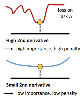
In this sense, the curvature of the loss landscape indicates the robustness of the minimum. A sharp region implies a low tolerance for parameter changes, while a flat region indicates greater flexibility. By using the FIM as a practical approximation of this curvature, EWC effectively estimates which parameters are essential to maintain previous performance.
Evaluation Protocols
The learning process is organized as a sequence of tasks, with specific procedures for training and testing:
- Training phase: The model learns tasks sequentially. At any time, it is trained only on the data of the current task. Once a task is mastered, typically using multiple epochs to ensure a proper fit, the model proceeds to the next.
- Testing phase: the model is evaluated on all tasks seen so far. The sequence of testing is irrelevant; the objective is to correctly classify all previously seen classes, regardless of their original task.
Hyperparameter Tuning and Cross-Validation: Currently, there are no universally established or common practices for tuning and validating CL models.
METRICS
To evaluate the model’s performance across the entire sequence of tasks, we utilize Average Accuracy.
Formally
Given a test set for each of the tasks, and indicating with the test classification accuracy on task after observing the last sample from task , we have:
In other words, it measures how well the model remembers each task after learning all tasks. It is commonly used to evaluate catastrophic forgetting: if the accuracy on a task drops significantly compared to when that task was first learned, it indicates that the model has forgotten previously acquired knowledge.
Although the formula refers to the accuracy at the end of the full sequence (), the metric can also be computed at any intermediate step during training.
Other metrics could be used, such as Backward and Forward Transfer (BWT and FWT)
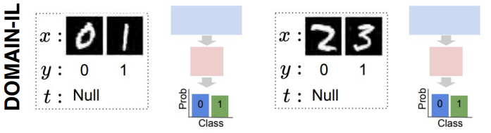
THREE SCENARIOS
Three main evaluation scenarios:
-
Task-Incremental Learning (Task-IL)
- Training: Tasks are learned sequentially.
- Testing: the task identity is provided for every test example. The model knows exactly which task the input belongs to and only needs to choose the correct class within that specific task’s output nodes.
- Difficulty: This is generally the easiest scenario because the search space is limited to the current task.
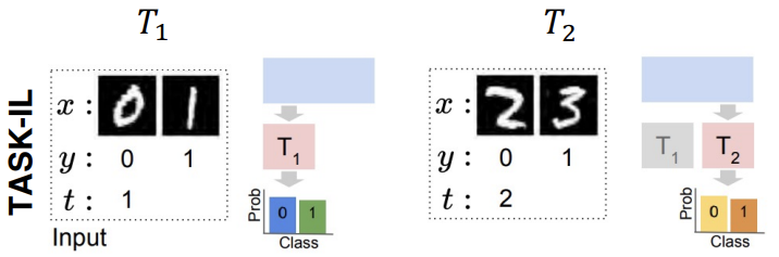
-
Class-Incremental Learning (Class-IL)
- Training: Tasks are learned sequentially, just like in Task-IL.
- Testing: The task identity is NOT provided. The model must classify the input correctly among all classes seen so far across all previous tasks.
- Difficulty: This is significantly more challenging than Task-IL. The model must not only distinguish between classes within a task but also avoid confusing classes from different tasks (inter-task confusion).
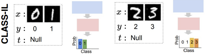
-
Domain-Incremental Learning (Domain-IL)
- Training: The set of possible classes (labels) remains fixed across all tasks.
- Testing: Each task introduces a domain shift (a change in the input distribution), but the target labels do not change.
- Examples: This is often simulated using data transformations, such as changing the background, weather conditions, or applying rotations/permutations to the inputs while the object to be classified remains the same.
A TAXONOMY OF CL APPROACHES
CL approaches are typically categorized into three categories:
- Architectural methods: mitigate forgetting by modifying the model architecture, often allocating distinct sub-models or specific parameters to different tasks.
- Regularization methods: introduce additional loss terms that constrain weight updates to preserve previously learned knowledge.
- Replay methods: maintain a small memory of past experiences and reuse them during training to remind the model of previously learned tasks.
Architectural approaches
WEIGHT SHARING
In standard Continual Learning, the model updates the same set of weights for every task. When Task B is learned, it modifies the parameters previously optimized for Task A. These updates overwrite the optimal configuration for past tasks, leading to catastrophic forgetting. This reliance on a single, shared parameter space is the primary driver of inter-task interference.
ARCHITECTURAL APPROACHES
To mitigate this interference, architectural methods introduce new weights tailored for new tasks instead of overwriting existing ones, thereby expanding the model’s capacity. The core idea is to allocate distinct sub-models or task-specific parameters to different tasks.
These approaches can guarantee maximal stability (zero forgetting) by freezing the parameter subsets associated with previous tasks, ensuring they are not overwritten.
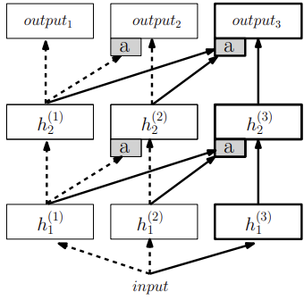
Progressive Neural Networks
Progressive Neural Networks (PNNs) are a foundational example of the architectural strategy. Instead of modifying a shared set of weights, PNNs prevent catastrophic forgetting by instantiating an entirely new neural network, referred to as a column, for each task.
The PNN architecture includes two main types of connections:
- Standard Connections: propagate information vertically within each column to solve the current task.
- Lateral Connections: connect the hidden layers of previous columns to the layers of the new column.
When learning Task B, the parameters of the column for Task A are frozen. The lateral connections allow the new column to access and reuse features learned from previous tasks, enabling knowledge transfer without overwriting existing knowledge.
ADVANTAGES AND LIMITATIONS
While Progressive Neural Networks offer a robust solution to forgetting, they involve significant trade-offs.
Advantages
- Accuracy (Zero Forgetting): Because the parameters for old tasks are never modified, the model is immune to catastrophic forgetting by design.
- Knowledge Reuse: The lateral connections allow the model to leverage “transfer learning,” utilizing old computations to help solve new problems without relearning basic features.
Disadvantages
- Scalability (Parameter Explosion): The number of parameters, and consequently the memory footprint, grows linearly with the number of tasks. This creates an intrinsic bound on how many tasks can be learned before hardware resources are exhausted.
- Limited to Task-IL: PNNs are generally restricted to Task-Incremental Learning (Task-IL) because, at inference time, the model must know the task identity to activate the appropriate column. This makes them unsuitable for Class-Incremental Learning (Class-IL), where the task origin of an input is unknown.
- Unidirectional Knowledge Sharing: Knowledge transfer occurs only from earlier tasks to later ones. As a result, earlier tasks cannot benefit from knowledge learned in subsequent tasks.
SOLUTION
To address the scalability issues of Progressive Neural Networks (PNNs), researchers observed that adding full columns often results in most of the new capacity being underutilized. Instead of increasing the network size, methods like PackNet, PathNet, and Piggyback manage existing capacity through techniques such as adding fewer layers, pruning, or performing online compression.
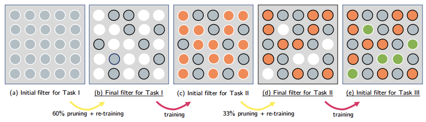
PACKNET
PackNet leverages the natural redundancies in large deep networks by “packing” multiple tasks into a single, fixed-size network. This minimizes performance drops and reduces memory usage, avoiding the parameter explosion observed in PNNs.
For each new task, PackNet follows a specific operational cycle:
- Train: The network is trained on the current task. Initially, all available weights are free to learn (represented in grey in the image).
- Prune: Weights with the smallest magnitudes are set to zero, freeing up capacity and creating a sparse mask for the task (white circles in the image b.).
- Retrain: The remaining weights are fine-tuned to recover any lost performance.
- Freeze: The weights used for this task are then frozen. Future tasks can only use the “pruned” (empty) connections.
Each task is associated with a binary mask that determines which weights are active during the forward pass. During inference, if the task identity is known, the corresponding mask is applied so only the weights allocated to that task are used.
All weights are effectively “packed” into a single network, while the masks control task-specific activation. This approach reduces memory usage and allows new tasks to be learned without overwriting previous ones.
Regularization approaches
Regularization methods integrate explicit terms into the loss function to balance the old and new tasks. These techniques encourage the model to maintain consistency with previously learned knowledge by comparing a current model against a reference (old) model.
While these approaches utilize weight sharing and do not instantiate additional parameters, thereby reducing the memory footprint, the regularization objective usually requires storing a frozen copy of the previous model for reference.
Depending on what part of the network is targeted, these methods are divided into two primary directions:
-
Weight regularization
Weight regularization methods constrain the variation of network parameters. This is often done using a quadratic penalty that penalizes changes to each parameter according to its importance for previous tasks:
- Important parameters are constrained more strongly to preserve knowledge.
- Less important parameters are allowed to change more freely to learn new tasks.
Examples include EWC, Synaptic Intelligence (SI), MAS, and RWalk.
-
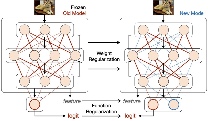
Function regularization
Function regularization targets the intermediate or final outputs of the prediction function rather than the weights themselves. This is commonly implemented through knowledge distillation, where the previously learned model acts as the “teacher” and the current model acts as the “student.”
Distillation can be applied at different levels:
- Feature-level distillation (matching intermediate activations)
- Output-level distillation (matching predicted probabilities)
Examples: Learning without Forgetting (LwF, next slides).
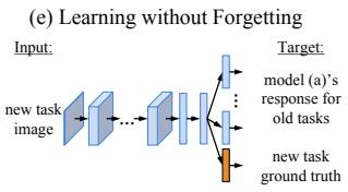
Learning without Forgetting (LwF)
A core challenge with distillation-based approaches is that matching a previous model’s output typically requires access to data from previous tasks. However, in many continual learning settings, past data is unavailable.
Learning Without Forgetting (LwF) addresses this by using data from the current task to approximate previous knowledge. The goal is to maintain performance on both old and new tasks using only new-task data.
THE PROCESS
LwF applies Knowledge Distillation (KD) between a “teacher” (the frozen network from the previous task) and a “student” (the current network learning the new task).
-
Generate Pseudo Labels: A new-task image is passed through the teacher network in a forward pass. The resulting output probabilities serve as pseudo labels, representing the knowledge of the previous model.
-
Dual-Supervision Training: The student network is trained on the new-task data using two distinct signals:
- True Labels: Standard supervision for the new classes.
- Distillation Supervision: the student is encouraged to match the teacher’s output probabilities for previously learned classes.
This approach assumes that the distribution of new data is not drastically different from past data, since the current data is used to approximate previous knowledge.
SUMMARY
Advantages:
- Bounded memory cost
- They can further distill knowledge on the large stream of unlabeled data that may be available in the wild
Disadvantages:
- Not very effective on long tasks
- Vulnerable to domain shift between tasks
To mitigate these disadvantages, a common solution is to provide a few training samples from old tasks, this transitions the strategy into Replaying Approaches.
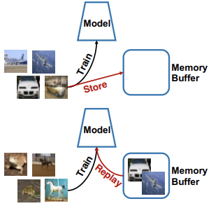
Rehearsal approaches
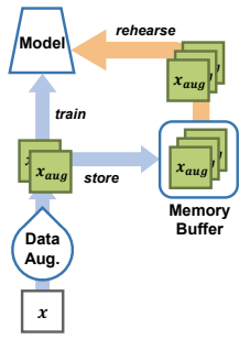
Rehearsal approaches mitigate catastrophic forgetting by storing a small subset of previously seen examples in a memory buffer and using them during later training iterations.
Procedure
Experience Replay (ER) maintains a memory buffer with a fixed capacity to store a limited number of old training samples and their corresponding labels. When training on a new task, the model is optimized using a combination of:
- Current Task Samples: Data from the task currently being learned.
- Replay Samples: A selection of samples retrieved from the memory buffer.
The buffer typically contains only a small fraction of the original data (e.g., 5-10% per class), making it significantly more memory-efficient than storing entire datasets. However, the model’s ability to retain past knowledge depends on the size of this buffer; larger buffers generally lead to better performance.
THE ER LOSS FUNCTION
The total loss is the sum of the cross-entropy loss calculated over both the current task distribution and the stored past data distribution:
This process acts as a form of rehearsal, where the model periodically revisits previously learned concepts while learning new ones, preventing the model from forgetting past tasks.
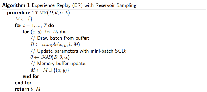
PSEUDOCODE
MEMORY ALLOCATION
Due to extremely limited storage space, the primary challenges in rehearsal involve how to construct and exploit the memory buffer. To recover past information in an adaptive way, stored samples must be carefully selected, compressed, augmented, and updated.
Naive Allocation Strategy
A simple solution is to divide the buffer into fixed portions assigned to each task. When a portion is full, older examples from that task are removed to make space for new ones.
However, this strategy has several limitations:
- It assumes the number of tasks is known in advance.
- It assumes tasks have similar importance and dataset sizes.
- Memory usage can become inefficient when only a few tasks have been observed.
For these reasons, most continual learning methods rely on dynamic sampling strategies.
SAMPLING STRATEGIES
Sampling strategies determine which samples should be stored in the buffer and which should be discarded, ensuring that the buffer remains a representative approximation of the entire data history:
-
Representative Samples store samples that best represent each class. A common approach is to use intermediate neural network features to identify samples that are closest to the class prototype or centroid in the feature space.
An example of this idea is the Mean-of-Feature strategy, which selects samples closest to the feature mean of each class.
-
Random Sampling If memory capacity is sufficiently large, randomly selecting samples is a simple yet effective way to approximate the original data distribution
-
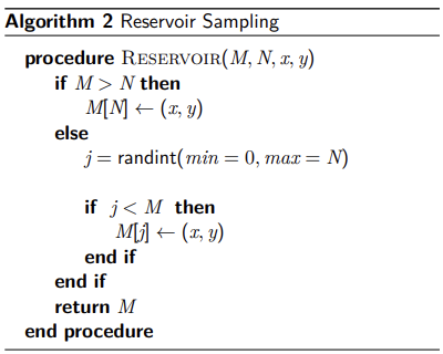
Reservoir sampling Reservoir sampling is a online version of random sampling that maintains a uniform sample of all observed data, even when the total number of examples is unknown in advance.
It ensures every item seen has an equal probability () of being in the buffer, where is the buffer size.
- If the buffer is not full: New examples are added directly.
- Once the buffer is full: A random decision determines if a new sample replaces an existing one.
Other sampling strategies
Several additional strategies have been proposed to improve the representativeness of the memory buffer:
- Ring Buffer: maintains a balanced number of stored samples per class.
- Weighted Reservoir Sampling: increases the probability of retaining more informative or difficult examples.
- Gradient-based strategies (e.g., Gradient Sample Selection, GSS): select samples that maximize gradient diversity.
- Clustering-based methods (e.g., k-means selection): store samples that best cover the feature space.
ISSUE
While Experience Replay (ER) is an ideal foundation for Continual Learning due to its simplicity, it faces several significant limitations:
- Overfitting the model repeatedly optimizes over a relatively small set of stored examples.
- Recency Bias Incrementally learning a sequence of classes implicitly biases the network toward newer tasks
To address this, many state-of-the-art methods combine Rehearsal with Functional Regularization (Knowledge Distillation).
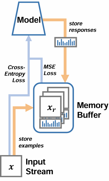
DARK EXPERIENCE REPLAY (DER)
Dark Experience Replay (DER) is a continual learning approach that leverages Dark Knowledge to retain past experiences. As the standard Experience Replay (ER), it maintains a subset of past data in a buffer . However, DER goes beyond simple rehearsal by storing not only input samples and ground-truth labels but also the model’s logits (outputs) at the time the sample was first processed.
The Training Objective
In addition to the current task loss (typically cross-entropy), DER introduces a regularization term to minimize the distance between current outputs and the stored past outputs:
where:
- Function Regularization: penalizes the Mean Squared Error (MSE) between current responses and stored responses , ensuring the model maintains its behavior on previous tasks.
- : A weighting factor that balances the preservation of past knowledge against the learning of the new task.
- : Indicates that the penalty is averaged across all samples stored in the memory buffer
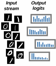
The logits stored in the buffer represent more than proxies for ground-truth labels: they capture the model’s knowledge at the time the sample was processed. Specifically, logits encode similarities and relationships between classes, providing a richer signal than discrete labels.
This process resembles knowledge distillation, where the current model is trained to reproduce the behavior of a previous model.
Learning without Forgetting (LwF) vs. Dark Experience Replay
This approach differs from methods such as Learning without Forgetting (LwF).
- Learning without Forgetting stores the previous model and uses it to generate targets for new training data.
- Dark Experience Replay instead stores data samples and their corresponding past outputs.
Both approaches aim to match the outputs of past and current models, but they differ in how this information is stored and used.
DER++
DER++ is a variant of DER that also asks the learner to predict the ground truth labels for past examples.
OTHER REHEARSAL APPROACHES
Other common rehearsal approaches:
- Gradient Episodic Memory (GEM) and its lightweight variant Average-GEM (A-GEM)
- Meta Experience Replay (MER)
- Incremental Classifier and Representation Learning (iCaRL)
- Learning a Unified Classifier Incrementally via Rebalancing (LUCIR)
- Approaches tailored to Vision Transformers (VIT):
- Learning-to-prompt (L2P)
Rehearsal-free approaches
PROBLEMS WITH REPLAY-BASED APPROACHES
Core issues:
-
Episodic Memory Constraints
These approaches require an episodic memory buffer to store raw samples or feature embeddings from previous tasks. This leads to two primary issues:
- Storage Costs: As the number of tasks increases, the memory required grows proportionally.
- Privacy Concerns: Storing past data is often unfeasible for sensitive data (e.g., medical or personal domains).
-
Selection complexity:
Determining which specific samples to store can strongly impact performance. The choice of strategy, whether using herding, class-balanced coresets, or reservoir sampling, significantly influences how well the model remembers previous tasks.
-
Distribution mismatch:
A limited buffer does not provide a faithful representation of the original data distribution. This mismatch often results in:
- Biased gradient updates during training.
- Catastrophic forgetting of underrepresented data modes.
As a result even large buffers, cannot fully replicate the effect of having full past data.
MOTIVATION FOR REHEARSAL-FREE CL
The limitations of replay-based methods have motivated the development of rehearsal-free approaches. These methods remove the need for explicit data storage, making them easier to deploy in privacy-sensitive settings and reducing the overall resource footprint.
By removing complex buffer management and sample selection strategies, rehearsal-free methods simplify the learning process, shifting the focus from remembering past data to preserving useful knowledge within the model. This is typically achieved by using a frozen backbone as a stable knowledge base, while new tasks are learned by adapting only small portions of the network.
Modern rehearsal-free CL methods often rely on pretrained foundation models (e.g., ViT, CLIP, T5) as this stable backbone. These models provide:
- Broad and general-purpose representations
- Robustness to distribution shifts
- High transferability across downstream tasks
ADVANTAGES
- Data Integrity and Privacy By eliminating the need to store raw data samples, these methods are ideal for sensitive domains. The memory acts as a repository of task-specific parameters (small vectors) rather than a collection of full data samples.
- Efficiency and Stability
- Parameter-Efficient Updates: Using prompts, adapters, or LoRA allows for targeted learning without large-scale gradient updates.
- Reduced Interference: Because the pretrained model remains unchanged, new learning is less likely to overwrite old knowledge, effectively limiting catastrophic forgetting.
- Better scalability These approaches scale more effectively to a large number of tasks or clients.
Recall Prompting
Prompting involves adding a small number of learnable tokens to the input prompt, which are optimized during training, while leaving all other backbone parameters frozen.
Each prompt token is a learnable -dimensional vector. A collection of prompts is denoted as:
When optimizing prompts with Shallow Prompt Tuning, the prompts are only applied to the first Transformer layer :
where:
- is the patch embeddings,
- represents the features computed by the -th Transformer layer,
- is the CLS token.
This approach is useful because it keeps the backbone frozen, reducing forgetting, while introducing only a small number of task-specific parameters that guide the model’s behavior. By keeping the backbone fixed and learning prompts as new parameters, the model achieves a good stability–plasticity trade-off, similar to PNNs, while adding only a negligible number of learnable parameters.
Challenge: an effective mechanism is required to select the appropriate prompts for each task; otherwise, this strategy cannot be applied in Class-Incremental Learning (Class-IL) scenarios.
PROMPTING STRATEGIES IN CL
Prompting strategies in CL:
- Task-specific prompts: one set of prompts per task.
- Dynamic prompt selection: reuse or combine prompts for new inputs.
- Prompt merging: combine previous knowledge into compact representations.
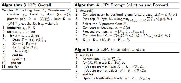
L2P: Learning to Prompt for Continual Learning
L2P aims to achieve strong continual learning performance without rehearsal and without requiring task IDs at inference (task-agnostic setting).
ARCHITECTURE
L2P utilizes a frozen ViT backbone and introduces the following components:
- Prompt Pool: A collection of learnable prompt vectors .
- Key-Query Matching: For every input, a query embedding is computed and compared with the learned keys associated with each prompt. The system then selects the top- prompts based on highest similarity.
- Classifier Head: A lightweight head updated for each specific task.
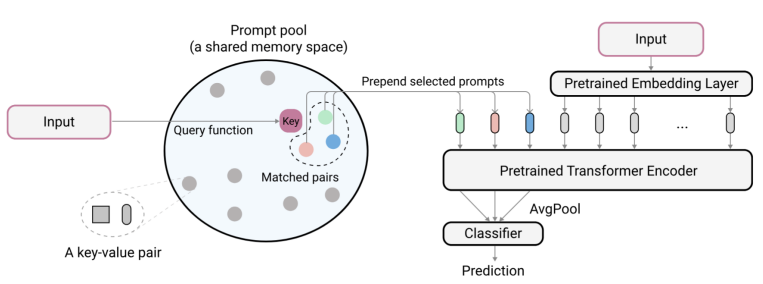
TRAINING AND INFERENCE
Training phase:
- Only the prompt pool and the classifier head are trained using task-specific data.
- The backbone weights remain entirely fixed.
Inference phase:
- The system retrieves the most relevant prompts dynamically based on the input query.
- The selected prompts are appended to the input and processed by the frozen backbone.
Because prompt retrieval depends on input similarity, the model does not require task IDs at inference, making it task-agnostic.
Intuition: different inputs retrieve different prompts, enabling flexible task adaptation without modifying the backbone.
ADVANTAGES AND LIMITATIONS
Key Advantages
- Rehearsal-Free: Operates without the need for a data buffer.
- Task-Agnostic Inference: Can identify the correct task-specific information without being provided a Task ID at test time.
- Parameter Efficiency: Only the prompts and the classifier head are updated.
- Scalability: Performs well as the number of tasks increases.
Current Limitations
- Capacity Tuning: The size and diversity of the prompt pool require tuning.
- Task Similarity: Performance may degrade if tasks are highly dissimilar.
- Pretraining Dependency: The effectiveness of the approach relies heavily on the quality and breadth of the pretrained foundation model.
Key Takeaways
| Concept | Description |
|---|---|
| Catastrophic forgetting | Standard SGD updates a shared weight set toward each new task’s loss, overwriting solutions for previous tasks |
| Continual learning (CL) | Train sequentially on a stream of tasks while preserving past knowledge — without retraining on the union of all data |
| Cumulative loss objective | — minimize loss across all tasks seen so far, without access to old data |
| Task-IL / Class-IL / Domain-IL | Three scenarios: task ID at test, no task ID with class space growing, fixed labels with shifting input distribution |
| Average Accuracy (ACC) | — accuracy across all tasks after the full sequence; primary CL metric |
| EWC | Quadratic penalty anchors important parameters; importance from the diagonal Fisher Information Matrix |
| Fisher Information | Approximates loss curvature; high = sharp minimum, weight matters → high penalty; low → free to move |
| Architectural methods | Allocate new parameters per task — zero forgetting by design (e.g., PNN, PackNet) |
| Progressive NN (PNN) | One frozen column per task with lateral connections for forward transfer; parameters grow linearly, Task-IL only |
| PackNet | Train → prune small-magnitude weights → retrain → freeze; pack many tasks into one fixed-size network via per-task binary masks |
| Regularization methods | Add a loss term that compares current model to a frozen reference — weight (EWC, SI, MAS) or function (LwF) |
| Learning without Forgetting (LwF) | Distill the previous model’s outputs on new data — no need to store old samples |
| Rehearsal / Experience Replay (ER) | Keep a small buffer of past samples; loss = current task + buffer cross-entropy |
| Buffer sampling | Reservoir sampling (uniform online), ring buffer (per-class balance), GSS (gradient diversity), mean-of-feature, etc. |
| DER / DER++ | Store inputs plus logits; regularize with MSE on logits (DER) and add CE on stored labels (DER++) |
| Rehearsal-free CL | No buffer — instead use a frozen pretrained backbone and learn small task-specific modules (privacy, scalability) |
| L2P | Frozen ViT + learnable prompt pool; key–query matching retrieves prompts per input → task-agnostic, rehearsal-free |
| Stability–plasticity trade-off | Core CL tension: keep old knowledge (stability) while adapting to new tasks (plasticity) |