Discrete AI
Introduction
DISCRETIZATION
While most deep learning models operate in continuous vector spaces, many real-world processes are naturally represented by discrete symbols. To better model these domains, we aim to build architectures that can learn discrete representations.
The Discretization is the process of partitioning continuous phenomena into distinct parts, this aligns closely with the way humans interpret and interact with the world.
Many real-world domains are inherently discrete, and modeling them with continuous representations may miss important structural properties. Common discrete domains include:
- Language consists of sequences of discrete symbols (words, subwords, or phonemes).
- Images are stored as discrete grids of pixels with quantized color values.
- Music and speech are often represented symbolically (e.g., notes, phonemes).
DISCRETE AI SYSTEMS
In the context of artificial learning systems, discrete models and representations enable:
-
Efficient compression The discrete latents are easier to encode compactly, so by utilizing a discrete domain, we can deploy highly efficient algorithms to compress complex data (such as images).
-
Symbolic reasoning classic logical reasoning (such as Boolean algebra) operates on discrete states.
-
Modular design Instead of processing every input through every layer (as in continuous projection), the model can use discrete signals to “route” inputs to specific sub-modules or transformations. This allows the network to dynamically choose which parts of the model to activate based on the specific input.
PROBLEMS
Neural networks are optimized using Gradient Descent, which relies on the chain rule of calculus to backpropagate error gradients. This requires every operation in the computational graph to be differentiable.
However, discrete operations break this pipeline because they are not differentiable. This creates several fundamental issues:
Case Study 1 — Quantization
Consider a function that maps a continuous value to the nearest integer:
Neural networks learn through gradients: during the backward pass we use gradients to update the weights. But quantization is not a differentiable function:
- Forward pass: Continuous inputs jump to discrete values (e.g., 1.4 → 1.0). Small changes in the input do not change the output, producing flat regions in the function.
- Backward pass: The gradient is 0 (because the curve is flat between steps). With a zero gradient, the network cannot update its weights, effectively blocking learning at this layer.
Case Study 2 — Hard Selection (Argmax)
A common discrete operation is selecting the “best” option from a set. This is often done using argmax which again is a non-differentiable operation. It selects an index, breaking the computational graph.
When backpropagation reaches an argmax, gradients cannot flow through it. To train such systems, we need strategies that produce a differentiable approximation of the maximum (e.g., softmax relaxations, Gumbel-Softmax, etc.).
Another challenge is that we do not always know which loss function is appropriate for training models with discrete components. Classical losses (like MSE or cross-entropy) assume differentiability, so new formulations are required when discrete choices are part of the model.
SOLUTIONS
We will see some solutions:
- VQ-VAEs involve straight-through estimators
- Pixel-RNN employ autoregressive training (teacher forcing, likelihood maximization)
- Surrogate gradients (e.g., Gumbel Softmax)
Vector Quantized-Variational Autoencoders
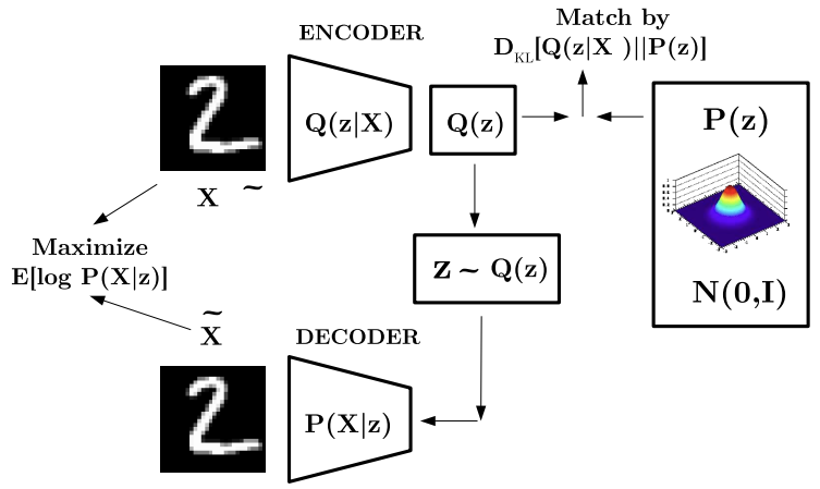
VARIATIONAL AUTOENCODER: OVERALL ARCHITECTURE
VAE: KNOWN ISSUES
-
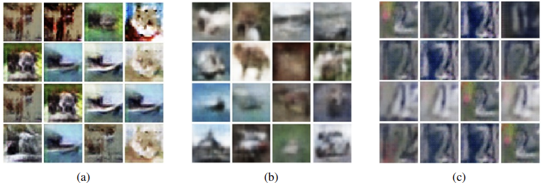
Blurry, low-quality outputs:
VAEs often produce outputs that look blurry or unrealistic. In many samples, the background tends to dominate and the generated images lack fine details.
-
Mode collapse:
The model may generate only a small subset of the possible outputs (i.e., a few “modes” of the data distribution), failing to capture the full diversity present in the training set.
VAE: PROBLEMS
The standard VAE formulation uses a Kullback-Leibler (KL) divergence term that forces the latent representations to approximate a standard Gaussian prior.
This pushes different inputs toward a single unimodal Gaussian distribution, reducing the expressiveness of the latent space and leading to overly smooth, blurry reconstructions. Ideally, the model should employ a more flexible, multimodal prior that better reflects the structure and variability of real-world data.
This strict regularization also leads to posterior collapse, where the encoder’s variational posterior quickly becomes identical to the prior during the early stages of training. When the KL penalty is too strong, the network learns that the “safest” strategy is to ignore the input and simply output the prior distribution. As a result, the latent variables stop carrying meaningful information, and the decoder learns to ignore them.
This collapse is often difficult to reverse: once the encoder converges to an uninformative prior, it rarely recovers without explicit intervention.
Solution(s):
-
β-VAE Introduces a hyperparameter that controls the weight of the KL divergence term in the ELBO objective:
-
Vector Quantised-Variational AutoEncoder (VQ-VAE)
VECTOR QUANTISED-VARIATIONAL AUTOENCODER (VQ-VAE)
VQ-VAE was the first successful generative model to use discrete latent variables. It utilizes the full latent space and completely avoids posterior collapse, because it does not use a KL term that forces the posterior toward a fixed prior.
It resembles a standard autoencoder with an encoder and decoder, but unlike VAEs, the latent embedding space is not Gaussian. Instead, it is composed of discrete learnable embeddings.
How does it work?
-
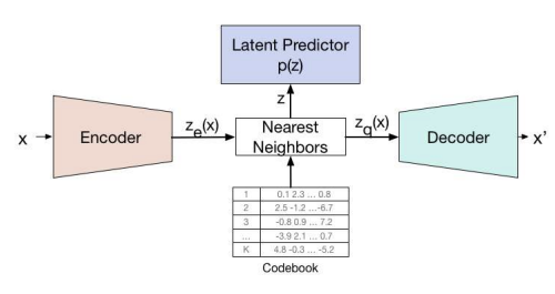
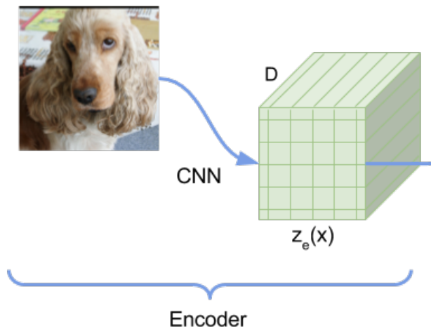
Encoding
The model takes an input image , which is passed through the encoder. This produces a continuous output where:
- width
- height
- channels
-
Codebook
The encoder output is mapped into a grid of discrete latent variables, through a learnable codebook (lookup table) , where:
- is the size of the discrete latent space (number of code vectors)
- is the dimensionality of each latent embedding vector.
The codebook consists of embedding vectors which can be learned through gradient descent.
The discrete indices used in the latent grid range from to .
-
Nearest-Neighbor Assignment (Quantization)
For each location in , the corresponding discrete latent index is obtained via nearest-neighbor lookup:
The proposal distribution is deterministic.
-
Decoder
The input to the decoder is the corresponding embedding vector :
The decoder takes this grid of discrete tokens and attempts to reconstruct the original image.
This quantization step is not differentiable.
VQ-VAE uses the straight-through estimator to allow gradients to flow.
The complete set of parameters are union of parameters of the encoder, decoder, and the embedding space .
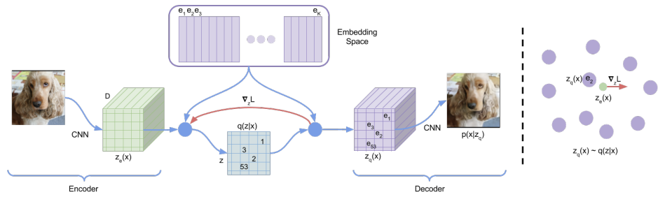
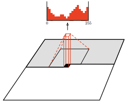
Figure 1: Left: A figure describing the VQ-VAE Right: Visualisation of the embedding space. The output of the encoder is mapped to the nearest point . The gradient (in red) will push the encoder to change its output, which could alter the configuration in the next forward pass.
VQ-VAE: LEARNING
The forward pass is like a standard autoencoder, but with a non-linearity that maps latents to a 1-of-K embedding vector. This operation is non-differentiable, as discrete functions like argmax, round, or quantize break gradient flow.
Solution: straight-through gradient estimation. To address this, gradients are approximated by copying them from the decoder input to the encoder output .
STRAIGHT-THROUGH GRADIENT ESTIMATION
The Straight-Through Estimator enables training with non-differentiable operations by:
- Using the discrete output during the forward pass.
- Backpropagating gradients as if the operation were the identity.
Formally:
- Forward: (e.g., nearest codebook entry)
- Backward: (treat as identity)
This approximation prevents gradient flow from breaking and is commonly used whenever a layer is non-differentiable.
Applications:
- Binary neural gates: forward as step, backward as sigmoid
- Neural architecture search, routing, and pruning
VQ-VAE: TRAINING OBJECTIVE
To learn the embedding space, VQ-VAE utilizes Vector Quantization (VQ), a dictionary learning approach. Due to the non-differentiable nature of quantization, the architecture employs Straight-Through Gradient Estimation during backpropagation.
The overall training objective is defined as:
Note: denotes the detach operator. It treats its operand as a non-updated constant during backpropagation.
Where:
-
Reconstruction term
Compare the decoder output with the original input and minimize their difference (e.g., L2 or cross-entropy). This term updates only the decoder parameters.
-
Vector Quantization (VQ) term
This term aligns the codebook embedding vectors with the encoder outputs, so with the corresponding real value.
-
We take the encoder output .
-
We perform a nearest-neighbor lookup in the codebook and obtain .
-
The VQ loss minimizes:
So it moves the Codebook vectors closer to the encoder outputs. Since the encoder output is detached (stopgrad), only the codebook is updated.
-
-
The third term (commitment) encourages the encoder to be committed to the selected codeword .
This term treats the codebook vector as the ground truth (target) and pulls the Encoder output closer to it. This ensures the encoder produces values that translate easily into discrete symbols.
| Loss term | Trains | Does NOT train |
|---|---|---|
| Reconstruction | Decoder | Codebook, Encoder |
| VQ term | Codebook | Encoder, Decoder |
| Commitment term | Encoder | Codebook, Decoder |
The VQ-VAE differs significantly from the standard Variational Autoencoder (VAE).
- Standard VAE: Relies on a fixed Gaussian prior (fixed before, during, and after training) and continuous latent space.
- VQ-VAE: Replaces the Gaussian distribution with a discrete codebook that describes the latent space. Unlike the fixed static prior of a standard VAE, the VQ-VAE learns the distribution of the discrete latent space (the prior) during training.
VQ-VAE: TRAINING STEP
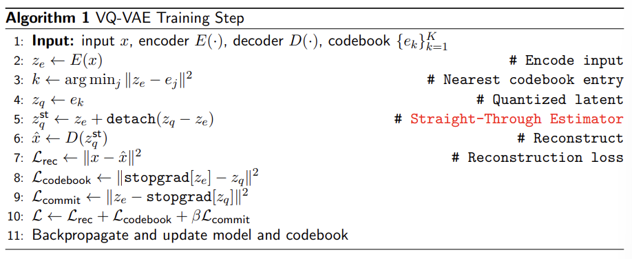
In PyTorch, the Straight-Through Estimator used in VQ-VAE can be implemented in a single line:
detach() breaks the computational graph, which means that during backpropagation
the term inside detach() is treated as a constant.
So:
-
During forward pass, you get the real quantized vector.
-
During backward pass:
Gradients stop at detach(), so only is considered and receives gradients.
Effectively the model pretends that:
→ quantization is treated as an identity function.
VQ-VAE FOR IMAGE COMPRESSION
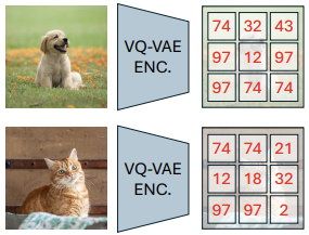
VQ-VAE can act as a learned image compressor:
- The encoder converts an image into a grid of discrete latent codes, which are far smaller than the original image,
- The decoder reconstructs the image from these codes.
- The resulting codebook indices can then be efficiently compressed using entropy coding methods such as Huffman or arithmetic coding.
This approach learns domain-specific representations, enabling higher-quality reconstructions at low bitrates compared to traditional handcrafted codecs.
SAMPLING FROM THE VQ-VAE LATENT SPACE
A VQ-VAE can reconstruct images, but it cannot generate new ones because it does not learn a prior over its discrete latent codes. Sampling random codebook entries would usually produce meaningless images, since the latent structure is unknown.
To solve this, we learn a prior over the discrete latent space (Learnable Prior). So instead of sampling directly from the discrete latent space, we first learn this distribution with another generative model.
The process:
- Prepare Data: Encode the original training data to obtain sequences of discrete latent codes. These sequences serve as the “ground truth” training set for the new model.
- Train Prior: Train a generative model (e.g., PixelCNN ) on these latent code sequences.
- Sample: After training, use the learned prior to sample a new sequence of latent codes. Each latent code corresponds to a specific spatial “patch” of the image.
- Decode: Pass the sampled codes through the VQ-VAE decoder to generate the final new image.
Autoregressive Models (PixelCNN)
Given a VQ-VAE codebook, our objective is to learn a distribution over sequences of discrete latent codes (symbols):
where:
In order to do so, we parameterize a generative model (a learned prior) using parameters . This defines a parametric distribution over sequences of discrete latent variables:
Where:
- denotes the total sequence length
- represents the size of the discrete vocabulary (the number of potential values for each symbol).
AUTOREGRESSIVE MODELLING OF DISCRETE LATENTS
Estimating the joint probability distribution of a set of random variables directly is often more complex due to the high dimensionality of the data.
To make this problem manageable, we apply the chain rule of probability, which allows us to rewrite the joint distribution as a product of conditional distributions. In this way, the prior over discrete latent codes can be learned using an autoregressive factorization:
This means that each latent code is predicted conditioned on all previous ones in the sequence.
For a sequence , this implies:
- depends on no prior context.
- is conditioned on .
- is conditioned on .
So we can rewrite the joint distribution as the product of conditional distribution:
CHAIN RULE OF PROBABILITY (BAYESIAN FACTORIZATION)
To justify the autoregressive factorization, we start from the fundamental product rule, which states that a joint distribution can be decomposed into a prior and a conditional probability:
Our goal is to apply this rule to the joint distribution of a sequence of random variables, . We can achieve the autoregressive factorization by recursively applying the product rule:
The derivation follows three logical steps:
- Isolation: We isolate the last variable, , and condition it on all preceding variables.
- Recursive Step: We repeat this process for the remaining joint term , “peeling off” one variable at a time.
- Termination: We repeat this exactly times until we reach the initial prior, .
This mathematical result is the definition of an Autoregressive Generative Model. It implies that the joint distribution can be written as a product of conditionals, where every random variable is conditioned only on its predecessors, not on future values.
Each latent variable is a discrete symbol from a codebook of size . Therefore, each conditional probability can be modeled as a categorical distribution over the possible codebook entries:
where:
- is the index of the selected codebook entry.
- is the predicted probability vector over each entry of the codebook, which can be parameterized by a neural network.
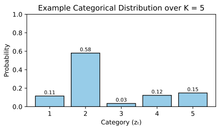
We can visualize this distribution as a histogram with bins. By sampling from this histogram, we determine the specific index for the next latent code .
Common choices for :
- Pixel Recurrent Neural Networks a recurrent neural network adapted to image data, where each pixel (or latent symbol) is predicted sequentially based on all previously generated ones.
- Transformer sequence models based on self-attention, which take the sequence of previous latent codes as input and output a categorical distribution over the possible symbols at each position.
- PixelCNN
PixelCNN
The general idea of Pixel CNN is that we can model the prior over discrete latent variables using a 2D autoregressive model implemented with a modified Convolutional Neural Network.
The joint distribution is factorized as:
where:
- is the pixel at row and column .
- denotes all pixels that come before position in raster-scan order (row by row, left to right).
Each conditional term is modeled as a categorical distribution predicted by a convolutional neural network.
Problem: The model must respect the autoregressive ordering: when predicting pixel , it must only access past pixels, never future ones. However, a standard convolutional kernel naturally looks at both past and future pixels in its receptive field, which breaks causality.
Solution: PixelCNN enforces autoregressive structure using masked convolutional kernels. As we will see later, a binary mask is applied to each convolutional filter so that all weights corresponding to future pixels are set to zero. This guarantees that the network is strictly causal during training and sampling.
INFERENCE
During inference, an autoregressive model such as PixelCNN generates an image sequentially, sampling one value at a time from the learned discrete probability distribution:
-
Initialization: Start with an empty image (or latent grid).
-
Sequential Generation: For each position in the image grid the model perform a forward pass through the PixelCNN to obtain the conditional distribution:
A new value is then sampled from this distribution:
-
Update The newly sampled value is inserted into the grid, and the process continues in raster-scan order (row by row and left to right).
Illustrative Example and Computational Cost:
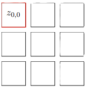
- For the first pixel (), the model learns a probability distribution that is not conditional on any previous data. Let us assume we sample a value, 128.
- This value (128) is fed back into the model to compute the distribution for the second pixel, conditional on the first. Suppose we sample 100.
- For the third pixel, the network evaluates the probability distribution conditional on both previous values (128 and 100).
This sequential dependency means that to generate an image of size , we must perform 100 separate forward passes during inference.
In this example: Each red square represents a forward pass and a sampling step.
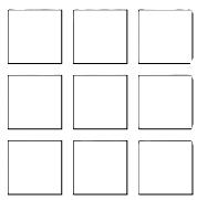
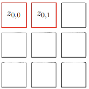
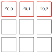
The process is repeated until the entire grid has been filled, meaning that all positions have been generated (all squares turn red).
Note: This sequential sampling procedure is inherently slow, since each pixel depends on all previously generated ones. As a consequence, sampling time scales linearly with the number of pixels, and pixel generation cannot be parallelized.
Conclusion: This method represents a clear trade-off: it provides a robust way to model discrete sequential distributions, but it is computationally expensive. It is a viable solution for short sequences or small grids, but it becomes impractical for high-resolution data due to the prohibitive inference time.
CAUSAL CONVOLUTIONS
So we said that in autoregressive models, we must ensure that the prediction at position depends only on previously generated positions. This prevents information leakage from future pixels (i.e., the model must not “see the future”).
To enforce this constraint, PixelCNN uses masked convolutions, which block access to all pixels that come after in the chosen ordering.
This is implemented by element-wise multiplying the convolutional kernel with a hard-coded binary mask. All weights that correspond to future positions are set to zero before each forward pass.
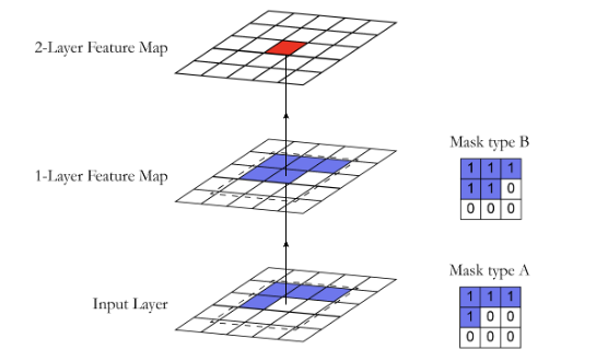
In practice, PixelCNN does not rely on a single mask, for 2D data (images), we have two masking strategies:
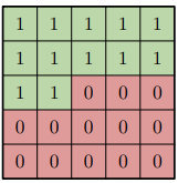
- Mask type A: is applied only in the first convolutional layer. It strictly excludes the current pixel from the calculation. This is necessary because is the target value we are trying to predict; if the model were allowed to see it in the first layer, the task would become trivial (identity mapping) rather than predictive.
- Mask type B: is used in all subsequent layers. Using the center pixel here is safe because the input to these layers is not the raw image, but a feature map. Therefore, allowing connection to allows the network to process and propagate this contextual information without violating the autoregressive constraint.
TRAINING
PixelCNN is trained to maximize the Log-Likelihood of the training data, which is equivalent to minimizing the Negative Log-Likelihood (NLL):
Since the model predicts a categorical distribution for each position (e.g., a softmax over categories, one for each line in the codebook), the training loss corresponds to the standard cross-entropy between the predicted distribution and the ground-truth class.
In practice, for each pixel , the model outputs a probability vector of size , whose entries sum to 1. Cross-entropy is applied independently at each location, encouraging the network to assign high probability to the correct class.
Problem: Sampling from PixelCNN is slow, as it requires a sequential forward pass for each pixel due to the autoregressive dependency. If we were to train the model in the same way—using its own generated samples to predict the next step—training would be computationally infeasible.
Solution: Teacher Forcing
During training, we already possess the ground-truth image. Instead of feeding the model its own sampled predictions from the previous step (as done in inference ), we feed the actual ground-truth pixels from the training data in the network.
This simple shift changes the computational paradigm:
- Parallelization: Since the input (the ground-truth image) is fully known, we can predict the distributions for all pixels simultaneously.
- Single Pass: The entire grid is processed in a single forward pass, rather than one pixel at a time.
This works even though the input contains “future” pixels, because the masked convolutions automatically prevent the model from accessing invalid information. As the convolutional filters slide across the image, the masks zero out all entries that correspond to future positions, ensuring the autoregressive constraint is respected.
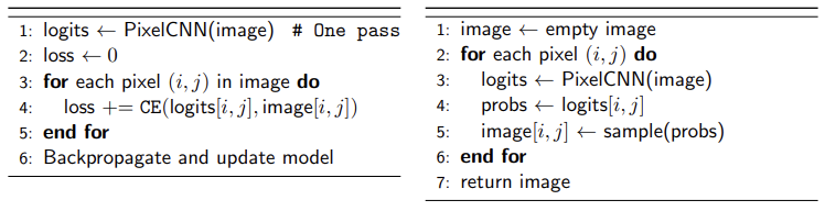
PSEUDOCODE
Training (single forward pass)
Sampling (autoregressive)
LIKELIHOOD AND ANOMALY DETECTION
PixelCNN models the exact data likelihood:
This allows us to assign a score probability (or log-likelihood) to any image:
- If the input truly comes from the training distribution (digits 1–4), this likelihood will be relatively high.
- If the input is unusual or unseen (e.g., a digit 5), the pixel-level probabilities will be small, and the overall likelihood will be very low.
This means PixelCNN can serve as a method for measuring how likely an input is with respect to the training dataset. By thresholding this likelihood, we obtain a simple but effective decision rule for identifying unexpected or out-of-distribution samples.
Applications
- Anomaly detection: Unusual images tend to have low likelihood under the model.
- Novelty detection: Detect out-of-distribution (OOD) samples by thresholding likelihood scores.
Key Takeaways
| Concept | Description |
|---|---|
| Discretization | Mapping continuous representations to discrete symbols; aligns with how humans interpret language, images, music |
| Non-differentiability problem | Discrete operations (argmax, quantize) have zero gradients, blocking backpropagation |
| VQ-VAE | Autoencoder with discrete codebook: encoder nearest-neighbor quantization decoder; avoids posterior collapse |
| Codebook | Learnable lookup table ; each entry represents a discrete latent concept |
| Straight-Through Estimator | Forward: use discrete output; backward: copy gradients as if identity. Implemented as |
| VQ-VAE loss | Reconstruction + VQ term (moves codebook toward encoder) + commitment term (moves encoder toward codebook) |
| Autoregressive factorization | ; chain rule decomposes joint distribution into sequential conditionals |
| PixelCNN | 2D autoregressive model using masked convolutions; learns a prior over discrete latent codes |
| Masked convolutions | Type A (first layer): excludes current pixel; Type B (subsequent layers): includes current pixel features |
| Teacher forcing | Train with ground-truth inputs instead of model predictions; enables parallel training via single forward pass |
| Gumbel-Softmax | Differentiable sampling from categorical distributions: ; temperature controls discreteness |
| VQ-VAE + PixelCNN pipeline | Train VQ-VAE (learn codebook) train PixelCNN on latent codes (learn prior) sample + decode |
Gumbel Softmax
We still face the same issue that appeared at the beginning of the lesson. When we sample from a distribution—e.g., by taking an argmax over logits during generation—the backward pass fails, because argmax is non-differentiable therefore gradients cannot flow through the sampling step.
PixelCNN suffers from exactly this problem during sampling: once we pick the most likely index from the histogram (the categorical distribution), this discrete choice breaks backpropagation.
STRAIGHT-THROUGH ESTIMATOR (STE)
In VQ-VAE, the trick used to handle the non-differentiable quantization step is the Straight-Through Estimator (STE). It works as follows:
- Forward pass: use the discrete codebook index selected by nearest neighbor search.
- Backward pass: ignore the discrete choice and copy the gradient from directly to , as if the quantization step were the identity function.
This works for VQ-VAE, but it is not suitable for sampling problems like those in PixelCNN, where the output is a categorical distribution, not a single codebook vector.
GUMBEL-SOFTMAX
The Gumbel–Softmax trick provides a differentiable way to sample from a categorical distribution inside a neural network, enabling backpropagation through the sampling operation.
Instead of performing a non-differentiable argmax or standard categorical sampling, the encoder produces logits over the possible categories. These logits are transformed into a soft sample using the Gumbel–Softmax relaxation:
Where:
- is the predicted probability of category ,
- are i.i.d. samples from a Gumbel(0,1) distribution,
- is a temperature parameter:
- , the samples approach a hard categorical distribution (one-hot vector).
- , the samples approach a uniform distribution.
Consider a scenario with Logits and Gumbel noise . The impact of reducing is evident:
- (Smooth): Output . The winner is distinct but the vector is “soft”.
- (Peaked): Output . The confidence in the first class increases.
- (Hard): Output . The vector is virtually identical to a one-hot encoding .
This mechanism closely resembles the reparameterization trick used in VAEs: the network provides logits (analogous to the mean in a Gaussian), noise is sampled from a known distribution (Gumbel instead of Gaussian), and the two are combined into a differentiable transformation.
DIFFERENTIABLE APPROXIMATION: FROM ARGMAX TO GUMBEL SOFTMAX
We can distinguish three approaches to sampling from a categorical distribution:
-
Hard categorical choice
This involves selecting the class with the highest probability:
Problem: It is non-differentiable.
-
Softmax:
This creates a continuous probability distribution, which is differentiable.
Problem: it’s not sampleable, it only gives probabilities.
-
Gumbel-Softmax (differentiable sampling):
To achieve differentiable sampling, we combine the Softmax function with Gumbel noise:
where:
-
This introduces stochasticity while keeping the operation differentiable with respect to the class probabilities
-
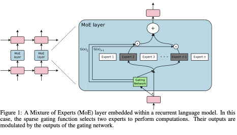
APPLICATIONS
Conditional computation refers to architectures where only a subset of the model is activated for each input, enabling sparse and efficient inference.
- It operates by selectively activating only parts of the network at a time.
- A common example is Mixture of Experts in large language model architectures.
Challenge: Selecting which computation path (e.g., which module or expert) to activate is typically non-differentiable:
Solution: Gumbel-Softmax Trick
- Provides a differentiable routing mechanism by producing a soft (or annealed-hard) one-hot vector.
- Allows the network to learn routing decisions via gradient descent, even though the final selection is discrete at inference.