Federated Learning
Introduction
Previously, we explored scenarios where tasks are distributed over time, such as Task 1, Task 2, and Task 3 appearing sequentially. In that setting, knowledge is acquired progressively as time passes.
We now shift our focus to a spatial distribution. Rather than appearing sequentially in time, tasks are distributed across different physical locations or devices simultaneously.
CENTRALIZED MACHINE LEARNING
In traditional machine learning, we usually assume a centralized setting, where:
- Unified Data Storage: All data is stored in a single location, giving the model access to the entire dataset.
- Single Model, Combined Dataset: A single global model is trained on this unified dataset. The training algorithm, the model, and its weights are all located on the same machine.
- Iterative Optimization (SGD): The model’s parameters are updated iteratively using Stochastic Gradient Descent, epoch after epoch, until convergence.
In this architecture, data, algorithms, and model parameters are consolidated at a single point in the network. While this setup is relatively simple to manage and avoids the complexities of distributed systems, it presents several limitations in real-world applications.
PROBLEMS
-
Data Privacy and Confidentiality
Handling sensitive data (e.g., medical records or personal communications) creates some privacy concerns. In many cases, regulations require that:
- Local Residency: Data must remain on the device where it was collected.
- Local Processing: Computations, including model training, must occur locally.
Because of legal regulations (such as GDPR or HIPAA), sending raw sensitive data to a central server is often restricted.
-
Infrastructure and Reliability
- Data Transfer Costs: Transferring large datasets from edge devices to a central server requires high bandwidth and can be expensive or impractical.
- Single Point of Failure: Centralized systems depend on a single central node. If it fails or the network connection is lost, the whole system may stop working.
-
Underutilization of Edge Resources
Centralized training relies only on the computational power of the central server, ignoring the capabilities of modern edge devices (such as smartphones or embedded systems) that could perform part of the computation locally.
SOLUTION: FEDERATED LEARNING
Federated Learning is a machine learning paradigm designed to address the limitations of centralized systems. Instead of collecting data in a single location, a central server coordinates a set of clients, such as mobile devices or organizations, to collaboratively train a model.
Each client contributes to the global model by sending learned knowledge, typically in the form of model parameters or weights, back to the server. In this way, sensitive raw data remains on the original device and is never shared.
By shifting computation to the edge of the network, Federated Learning improves both data privacy and operational efficiency.
FORMULATION
- Client-side: Each client holds a private dataset . The objective is to obtain the set of weights to minimize the loss using only its own dataset:
- Server-side: The server does not have access to the data; it only receives model parameters from the clients. Its objective is to obtain a global model that minimizes the average loss across the datasets of all clients:
APPLICATION SCENARIOS
-
Cross-device Federated Learning:
A large number of user devices (e.g., smartphones or IoT devices) each hold small amounts of data and collaboratively contribute to training a shared model.
- Example: training a mobile keyboard prediction model directly on users’ phones without uploading their keystrokes.
-
Cross-silo Federated Learning:
A smaller number of organizations (or silos) each possess richer local datasets and collaborate to train a common model.
- Example: multiple hospitals jointly train a diagnostic model without sharing patient records.
WEIGHT AVERAGING & MODEL MERGING
- The server maintains an initialized global model, while the data remains distributed across the clients.
- The server sends the global model to a subset of selected clients.
- Each client performs local training on its private dataset for one or more epochs.
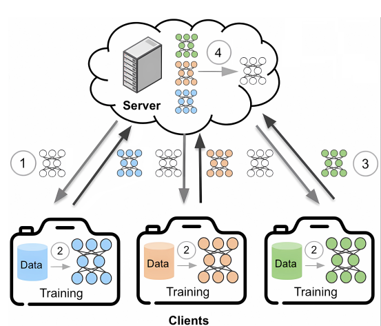
- After local training, clients send their model updates (e.g., gradients or updated weights) back to the server.
- The server aggregates these updates, typically by averaging them, to improve the global model. The goal is to obtain a model that performs well across all client datasets, even though the server never accesses the raw data.
- The updated global model is then sent back to the clients and used as the initialization for the next training round.
These steps are repeated until the model converges.
KEY CHALLENGES in FL
- Data heterogeneity (non-IID data): Clients often have data drawn from different distributions. This heterogeneity can cause client drift and may reduce the accuracy of the global model.
- Partial participation: In each training round, only a subset of clients participates. The set of active clients can change over time due to stragglers or device dropouts.
- Communication overhead: Network capacity is limited, so reducing the size and frequency of model updates is essential for maintaining efficiency.
- Privacy and security: Although raw data stays local, shared model updates may still leak information.
FAMILIES OF FL APPROACHES
- Baseline Method: Federated Averaging (FedAvg) – simple periodic averaging of local models to update the global model.
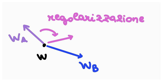
- Client-side Regularization: introduces constraints or adjustments during local training to reduce divergence across clients (e.g. FedProx, SCAFFOLD)
- Server-side Modifications: Adjustments applied at the server to improve convergence of the global model (e.g. Server Momentum, GradMA, Fisher-Averaging)
- Knowledge Sharing: Exchanges intermediate knowledge instead of raw model parameters (e.g. distillation-based methods, FedProto)
- Personalization: Tailors models to individual clients through fine-tuning or client-specific updates.
Federated Averaging (FedAvg)
Federated Averaging (FedAvg) is the foundational algorithm for Federated Learning. In this iterative process, a central server coordinates multiple rounds of training across a subset of clients. Each round, clients receive the global model, train it locally, and send only the updated parameters back to the server.
ALGORITHM
The process follows these steps:
- Initialize: Server sets initial global model parameters .
- Iterative Rounds: For each round :
- Server selects a subset of available clients.
- Server sends the current model to all clients in .
- Each client initializes the model and performs local training (e.g., epochs of SGD on its local dataset) to obtain an updated model .
- Clients send its model’s weights (or the model difference) back to the server.
- Server aggregates the weights to form the new global model:
- : model parameters from client at round .
- : number of training samples on client .
- : total number of samples across all participating clients in the current round.
This aggregation corresponds to a weighted average, where clients with larger datasets contribute more to the global model.
STRENGTHS AND LIMITATIONS
FedAvg has become the de facto baseline for federated learning experiments due to its practical advantages. It is simple to implement and reduces communication overhead by performing multiple local SGD steps per round instead of requiring frequent synchronization.
FedAvg performs well when client data is Independently and Identically Distributed (IID). However this assumption is frequently violated in real-world federated settings. When data is non-IID, local models can diverge significantly, a phenomenon known as client drift. This divergence can degrade both the convergence speed and the final accuracy of the global model.
One common form of non-IID data is label distribution skew, where different clients observe entirely different subsets of classes:
- Client 1: Observes only classes 1 and 2.
- Client 2: Observes only classes 3 and 4.
- Client 3: Observes only classes 5 and 6.
POSSIBLE IMPROVEMENTS
To mitigate these issues, researchers have developed various enhancements to the original FedAvg algorithm. These approaches can be roughly categorized into 3 families:
- Server-Side Approach: The server employs more powerful ways, instead of simply using the average, to aggregate the parameters.
- Client-Side Approach: Each client has some additional terms, e.g. regularization terms, that constrain their objective or their weights to force consistency w.r.t. the server.
- Prototype-based Approach: Constraints are forced in feature space instead of weight space, in order to obtain a good trade-off between consistency among clients and specialization on local-datasets.
Server-side Approach
Standard parameter averaging (such as FedAvg) treats every weight dimension as equally informative. While this is effective for i.i.d. data, it can be sub-optimal under data heterogeneity (non-i.i.d. settings).
An improved server-side strategy weights the contribution of each model parameter according to its importance for each client. Instead of relying only on dataset size, the server considers the model’s “confidence” in each parameter, quantified using the Fisher Information Matrix (FIM).
FISHER INFORMATION MATRIX
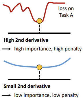
There is a theoretical relationship between the empirical FIM and the second derivative of the loss near a minimum. This reflects how sensitive the loss is to changes in a specific parameter:
- High Fisher Value (High Importance): A high value indicates a steep curvature. If parameter is pivotal, even minor modifications are likely to significantly increase the loss. Therefore, its value should be preserved more strictly in the global model to maintain client performance.
- Low Fisher Value (Low Importance): A low value indicates the parameter lies in a “flat” region of the loss landscape. If parameter is less vital, the server can modify or average it more freely, as changes will not drastically impact the loss.
By capturing the curvature of local objective functions, this approach allows more precise global updates, protecting parameters that are vital for local accuracy while permitting flexibility in less sensitive areas of the model.
FISHER-WEIGHTED AVERAGING
To aggregate models intelligently, we can treat each client’s weights as a probability distribution. Given client models with identical initialization, we approximate each model’s posterior as a Gaussian-distributed posterior:
where:
- is the Fisher Information Matrix, acting as a proxy for the model’s confidence.
The Optimization Objective
The objective is to find the set of weights that maximizes the joint posterior across all clients:
To simplify the computation, we apply a log transformation, converting the product into a summation:
In this context, are scalars (where ) that represent additional importance weighting, such as or proportional to dataset size.
The Closed-Form Solution
Solving this optimization problem leads to a specific closed-form solution for the global model parameters:
This approach mirrors the logic of Bayesian Neural Networks (BNNs). By modeling weights and their importance, the FIM effectively dictates the “certainty” of a parameter.
Addressing Computational Complexity
Problem Estimating and storing a full FIM is often unfeasible for modern, over-parameterized neural networks due to the massive number of parameters.
Solution We can use a diagonal approximation of the FIM. Representing the matrix as a vector makes the computation tractable.
For each individual parameter , the solution simplifies to:
If all importance scores are equal (), this formula reduces exactly to standard Federated Averaging.
PRACTICAL CONSIDERATION IN FL
Each client must transmit two primary components to the server:
- The updated local model weights
- The diagonal Fisher vector calculated after local training using the squared gradient of the log-likelihood on a local mini-batch.
Since both components have the same size as the model, the total payload per communication round is doubled. Although this increases bandwidth requirements, it remains practical in many Federated Learning settings where the model size is manageable.
From a privacy perspective, the Fisher values reveal only the sensitivity of the model parameters, not the raw data. However, they may still leak some information, so they are often combined with secure aggregation or differential privacy (DP) mechanisms.
STRENGTHS AND LIMITATIONS
Strengths
- Improves accuracy over FedAvg on heterogeneous data by weighting parameters according to their importance.
- Often performs even better when applied to pre-trained models, where clients share a common feature representation.
- Naturally supports one-shot federated learning or sporadic client participation, allowing models to be merged without multiple training rounds.
- Compatible with other server-side techniques, such as momentum or quantization.
Weaknesses
- Requires additional client-side computation, since multiple forward and backward passes are needed to estimate the FIM accurately.
- Can suffer from numerical instability, as the FIM may produce very large or very small values.
- May provide limited benefit when client models are too far apart in parameter space, because the FIM estimated on local data may no longer be meaningful at a very different point in the weight space.
DERIVATION OF FISHER-WEIGHTED AVERAGING
Setup
After local training, each client provides:
- the vector of model parameters, where is the number of parameters.
- the Fisher Information Matrix, which is symmetric and positive semi-definite.
Assume a Gaussian posterior around each . The goal is to find the parameter vector that maximizes the product of these independent posteriors:
This is equivalent to maximizing the sum of the logarithms of the posteriors:
Derivation
Assuming a Gaussian posterior with precision matrix :
The normalization constant does not depend on , so it can be ignored in the optimization:
Taking the logarithm and substituting into the objective:
Multiplying by yields an equivalent minimization problem:
Expand the quadratic forms:
The last term is independent of , so it can be removed from the optimization problem.
Collect terms
Collect as it does not depend on the summation over client models:
Take the gradient and set to zero
Since all are symmetric, we can write it as:
Solve for
If is the diagonal of the Fisher Information Matrix, we can treat it as a vector, that is . So the matrix inversion becomes a simple fraction (element-wise for each component ):
If all importance scores are equal (i.e., is the identity matrix for all clients) and represents the sample fraction per client, the solution reduces exactly to Federated Averaging (FedAvg).
Client-Side Approach
THE CLIENT DRIFT PROBLEM
In non-IID settings, FedAvg’s local updates often move in inconsistent directions because each client optimizes toward its own local optimum. Simply averaging models, even with importance weighting, may produce a global model that drifts away from the true optimum. The Key Drivers of this Drift are:
- Data Heterogeneity: the more dissimilar the clients’ data are, the more divergent the updates.
- Partial Participation: When only a subset of clients updates the model in each round, the global model’s trajectory becomes even more unstable, worsening the drift effect.
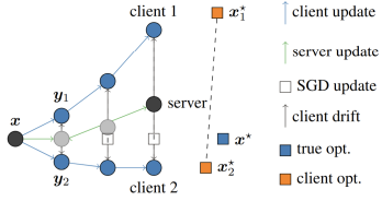
The primary result of client drift is either slower convergence or a suboptimal global model that fails to generalize effectively across all clients. This highlights a critical need: finding mechanisms to align local updates with the global objective.
SIMULATING THE IDEAL UPDATE
To mitigate client drift, the goal is to ensure each client follows the ideal update direction—the trajectory the model would take if all data were consolidated in a single central location.
This ideal direction could theoretically be achieved if clients transmitted both their model parameters and gradients to a central server. The server would then:
- Aggregate all local gradients.
- Compute a unified global update.
- Broadcast this correction back to the clients.
By using this global information, clients could adjust their local update direction, avoiding drift caused by non-IID data.
Challenge While this method would align local updates with the global objective, directly exchanging gradients is communication-expensive. The primary challenge, therefore, is to approximate this global correction efficiently.
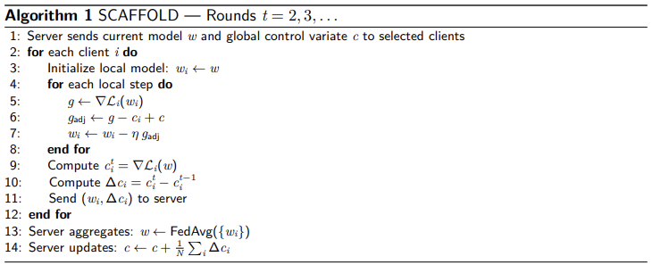
Scaffold
SCAFFOLD addresses the client drift problem by modifying the local update step. It incorporates a correction term—known as a control variate—to align local gradients with the global objective.
The algorithm introduces two auxiliary variables to track training directions:
- (Server Control Variate): An estimate of the global update direction (the path the model would take if all data were centralized).
- (Client Control Variate): A term that captures how client ’s local updates systematically differ from the global direction due to its specific local data distribution.
THE TRAINING PROCESS
Round 1: Initialization
- Initial Training: In the first round, no correction is applied; clients train normally on the initial global model .
- Local Estimation: At the end of the round, each client computes its initial (the average gradient experienced during local training) and sends it to the server.
- Global Aggregation: The server aggregates these values to form the global control variate:
Round 2 and Beyond: Corrected Training
When client receives the current global model , it no longer uses the raw local gradient . Instead, it applies an adjusted gradient:
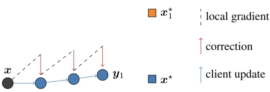
This formula works by:
- Removing local bias (): Subtracting the client’s own typical drift.
- Injecting global direction (): Adding the estimate of the ideal global path.
By using the signal , each client biases its optimization trajectory toward areas where there is stronger agreement among all participants.
Strengths and Benefits
- Mitigation of Client Drift: By constraining local updates to align with the global trajectory, SCAFFOLD keeps the model on a stable path toward the true optimum.
- Faster Convergence: Reduces variance between client updates, enabling provably faster convergence than FedAvg, especially under partial participation.
- Robust Regularization: Particularly effective in non-IID or challenging scenarios, where FedAvg might struggle or converge to a suboptimal model.
Limitations
- Scope of Impact: Client-side regularization alone may not suffice in complex settings. Server-side strategies, such as Fisher-weighted aggregation, may still be necessary to further improve performance.
Prototype-based Approach
Model or gradient averaging (like FedAvg) often proves suboptimal when client data distributions are highly divergent—for instance, when each client possesses data for entirely unique classes.
The Prototype-based approach addresses this by sharing interpretable intermediate representations rather than raw model parameters.
What is a Prototype?
A class prototype is a feature vector that captures the essence of a specific class from a client’s data. It is generated as follows:
- Feature Extraction: A neural network maps input examples into a high-dimensional embedding space.
- Clustering: Examples from the same class form a cluster in this space.
- Centroid Calculation: The prototype is defined as the centroid of these points. This is typically computed as:
- The mean of all feature vectors for that class.
- The medoid i.e., the point minimizing total distance to others in the cluster.
Prototypes can be used for classification (nearest prototype) and semantic alignment between clients.
The core hypothesis is that by sharing and aligning these prototypes, clients can build a consistent global understanding of each category.
- Improved Generalization: The global model learns what each class “looks like” by observing the average representation across clients, without accessing raw data.
- Handling Heterogeneity: Even if clients see completely different classes (e.g., Client A sees only dogs, Client B sees only cats), sharing prototypes allows all clients to build a consistent understanding of the full feature space.
FEDPROTO ALGORITHM
FedProto is a specialized federated learning framework that communicates through prototypes rather than model parameters.
The Training Process
For each client , the model is composed of a feature extractor and a classifier . The algorithm proceeds as follows:
- Local Prototype Computation At the end of each local training round, client calculates a prototype for every class present in its local dataset . The prototype is the mean feature embedding for each class in its local data:
-
Communication and Aggregation
Instead of full model weights, clients send these local prototypes to the central server. The server then averages them to form global prototypes () for each class.
-
Prototype Regularization
The server sends the global prototypes back to the clients. To ensure that local feature representations align with the global one, each client adds a regularization term to its local loss function:
effectively addressing the challenges of heterogeneous label distributions.
Inference: Nearest-Mean Classification
FedProto supports standard classifiers (e.g., softmax or linear heads trained with the local loss + regularization). Alternatively, a nearest-mean classifier can be used:
The input is assigned to the class whose prototype is closest in feature space, implementing a nearest-prototype classification strategy.
BENEFITS AND RESULTS
- Efficiency: Prototype vectors are much smaller than full model updates, reducing communication costs since only prototypes—not entire models—are shared.
- Effectiveness: Regularizing local models toward global prototypes allows FedProto to outperform FedAvg and similar methods on heterogeneous benchmarks, achieving higher accuracy.
Experiments demonstrate faster convergence and improved handling of clients with non-overlapping class distributions, making FedProto a simple yet powerful method for sharing knowledge beyond raw parameter averaging.
APPLICATIONS
-
Standard Federated Learning:
By optionally combining prototype sharing with parameter merging techniques (e.g., FedAvg), FedProto can learn a single global model like other FL methods.
-
Personalized Federated Learning:
Class prototypes allow each client to fine-tune its model locally while still benefiting from knowledge transferred through the prototypes.
-
Model-Heterogeneous Federated Learning:
Since prototypes are architecture-agnostic, FedProto works even when clients have different model architectures, unlike standard parameter-wise methods.
Summary and Conclusions
Federated Learning (FL) provides a robust framework for collaborative model training on decentralized data. By shifting the training process to the network’s edge, it addresses critical privacy, regulatory, and bandwidth constraints that typically make data centralization impractical.
While FedAvg serves as the simple and effective baseline for the field, its performance often degrades when client data is heterogeneous. This has led to the development of several sophisticated categories of enhancement:
- Client-side tweaks: e.g. FedProx, SCAFFOLD introduce regularization or control variates to reduce client drift.
- Server-side tweaks: e.g. Fisher-merge, introduce per-parameter weights to have a more fine-grained aggregation.
- Knowledge sharing: e.g. FedProto shares prototypes (or other knowledge) instead of raw model parameters to align learning.
These approaches greatly improve convergence speed and final accuracy in challenging FL settings (non-iid data, few clients per round, etc.), narrowing the gap between federated and centralized training.
FUTURE DIRECTIONS
As Federated Learning continues to evolve, research is shifting toward making these systems more robust and adaptable for real-world deployment. Key areas of focus include:
- Personalization: Moving beyond a single global model — allowing client-specific models or fine-tuning — is a key research direction to handle diverse user needs.
- Privacy enhancements: Incorporating stronger privacy guarantees (differential privacy, secure aggregation, etc.) without sacrificing too much accuracy remains an ongoing challenge.
- Scalability: Future FL systems must scale to millions of devices; this entails reducing communication (e.g., model compression) and handling unreliable devices and network conditions.
Overall, FL is key to enabling collaborative AI on distributed data. Ongoing research aims to make it more robust, fair, and applicable to a wider range of real-world scenarios.
Key Takeaways
| Concept | Description |
|---|---|
| Federated Learning (FL) | Train a shared model across clients without centralizing raw data; only parameters/updates are exchanged |
| Cross-device vs cross-silo | Many small/intermittent devices vs few organizations with rich datasets — different scale, reliability, and privacy regimes |
| Global objective | — average loss across all client distributions |
| Key challenges | Non-IID data, partial participation, communication overhead, residual privacy leakage from updates |
| FedAvg | Each round: server broadcasts → clients run epochs of SGD → server returns weighted average |
| Client drift | Under non-IID data each client moves toward its own optimum; averaging produces a model far from the joint optimum |
| Fisher-weighted averaging | Weight each parameter by client confidence (diagonal FIM): . Reduces to FedAvg when are equal |
| Diagonal FIM trick | Estimating the full FIM is infeasible; the diagonal — squared gradients of the log-likelihood — is a tractable proxy for parameter importance |
| SCAFFOLD | Client-side correction via control variates: replace with to align local updates with the global direction |
| FedProto | Communicate class prototypes (mean feature embeddings) instead of weights; regularize local features toward global prototypes |
| Prototype-based inference | Nearest-mean classification: . Architecture-agnostic, low communication cost |
| Three families of FL | Server-side (e.g., Fisher merging), client-side (FedProx, SCAFFOLD), knowledge-sharing (FedProto, distillation) |
| Privacy add-ons | Updates can leak; combine FL with secure aggregation and differential privacy for stronger guarantees |