Reinforcement Learning
Introduction
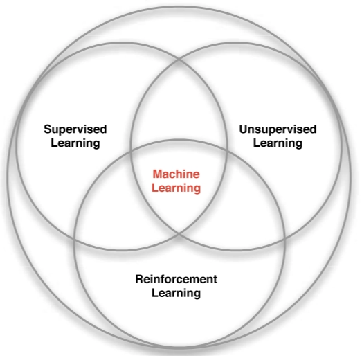
Reinforcement learning (RL) is a third paradigm in machine learning, alongside supervised learning and unsupervised learning.
- Supervised Learning: Relies on labeled data where each input is paired with a correct output. It is generally the most effective approach when labels are readily available.
- Unsupervised Learning: Operates on raw, unlabeled data to extract patterns or representations.
- Reinforcement Learning: Differs from both paradigms, because it operates without labels or prior knowledge of the “correct” action. Instead, an agent learns through trial and error by interacting with an environment to maximize cumulative rewards.
KEY CHARACTERISTICS
RL is defined by several unique attributes that distinguish it from other paradigms:
- No Labeled Supervision: The agent does not know the optimal action in advance and receives no explicit instructions on right or wrong moves.
- Reward Signal: The agent receives a scalar feedback signal, , indicating how well it is performing at step . Actions leading to high rewards are reinforced, while those leading to low or negative rewards are discouraged.
Helicopter Stunt Maneuvers: A positive reward is granted for following a desired trajectory, while a negative reward is issued for crashing.
- Delayed Feedback: Consequences may not appear immediately, making it difficult to determine which specific action was beneficial.
- Sequential Data: data is non-i.i.d. (independent and identically distributed), meaning that the current actions influence future states.
- Active Agency: The agent is an active participant whose actions directly affect the environment he lives in.
Inside a RL agent
SEQUENTIAL DECISION MAKING
The objective of the agent is to select actions that maximize the cumulative reward over the course of an episode. This requires considering the long-term effects of decisions, since:
- Actions may have long-term consequences.
- Rewards may be delayed.
- It may be beneficial to sacrifice an immediate reward in order to obtain a greater reward later (e.g., refuelling a helicopter now to prevent a crash several hours later).
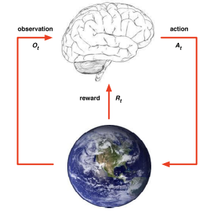
AGENT-ENVIRONMENT INTERACTION
The interaction is a continuous cycle defined by discrete time steps. At each step :
The Agent:
- Receives an observation (the current state of the environment).
- Receives a scalar reward
- Executes an action based on that information.
The Environment:
- Receives the action
- Transitions to a new state and emits the next observation
- Emits the next scalar reward
An episode represents a complete sequence of these interactions, from the initial state to a terminal state (such as the end of a game or the completion of a flight).
State
HISTORY
The history, , is the complete record of all interactions from the start of an episode up to the current time step . It includes the entire sequence of observations, actions, and rewards:
STATE
The state, , represents the specific information required for the agent to determine its next action. Formally, the state is a function of the history:
Although the current state depends on the entire sequence of previous interactions, using the full history is usually impractical. In practice, the state is a simplified representation that captures only the essential information needed for decision-making.
AGENT AND ENVIRONMENT STATES
In reinforcement learning, it is critical to distinguish between the internal state of the agent and the external state of the world:
- Agent state : the internal representation of information that the agent uses to select its next action. In most RL contexts, the term “state” refers specifically to this agent-side information.
- Environment state : the full configuration of the environment, the actual data the world uses to determine the next observation or reward. This state is typically invisible to the agent.
OBSERVABILITY
The relationship between these two states defines the nature of the learning task:
- Full observability: agent directly observes environment state, meaning
- Partial observability: agent only indirectly or partially observes the environment state (e.g., a poker agent sees only public cards, not opponents’ private cards).
RL systems generally do not attempt to explicitly model the complete environment state () for several practical reasons:
- Complexity: the environment may be too large or intricate to represent completely.
- Uncertainty: some underlying rules or variables may be unknown.
- Infeasibility: precise modeling can be computationally expensive and often unnecessary.
Instead, the agent learns through interaction and experience.
MAJOR COMPONENTS OF RL AGENT
An RL agent may include one or more of the following components:
- Policy: the function that defines the agent’s behaviour.
- Value function: estimates how good a state and/or action is.
- Model: a representation of the environment.
Policy
The policy defines an agent’s behavior. It acts as a mapping from state to action, essentially It determines which action the agent chooses in each state. Policies generally fall into two categories:
-
Deterministic policy
A deterministic policy maps each state directly to a single, specific action:
Example: in a specific state, the agent is programmed to always move left.
A purely deterministic policy can be impractical in complex environments, as it may require the agent to have pre-memorized the optimal action for every possible state it might encounter.
-
Stochastic policy
A stochastic policy defines a probability distribution over the available actions given a specific state:
Rather than choosing one fixed action, the agent assigns probabilities to all possible moves.
Return
The Return () is the total discounted reward starting from time-step :
The discount factor determines the present value of future rewards. Specifically, the value of receiving a reward after time-steps is . This mechanism prioritizes immediate rewards over delayed ones.
In reinforcement learning, future rewards are usually discounted, meaning rewards received further in the future contribute less to the total value. If the discount factor is close to:
0makes the agent myopic, valuing immediate rewards much more than future rewards,1makes the agent far-sighted, giving nearly equal importance to immediate and long-term rewards.
Value function
The value function tells us how good it is to be in a certain state under a given policy. There are two primary types of value functions:
- State-value function : the expected return starting from state and then following policy :
The agent evaluates the quality of its current state.
- Action-value function : the expected return starting from state , taking action , and then following policy :
Evaluates the quality of taking a specific action in a state.
While the state-value function evaluates the state itself, the action-value function allows the agent to compare the long-term impact of different individual actions within that state.
BELLMAN EXPECTATION EQUATION - STATE VALUE FUNCTION
The state-value function can be decomposed into two parts:
- The immediate reward received after taking an action in state ,
- The discounted expected value of the successor state
Formally, the equation is expressed as:
Derivation
We begin with the definition of the state-value function:
Substituting the definition of the return as the sum of discounted rewards:
Factoring out the discount factor :
The term inside the parentheses is the definition of the return at the next time step, :
Using the linearity of expectation:
Applying the law of iterated expectations:
Since , we obtain:
This is the Bellman expectation equation for the state-value function.
BELLMAN EXPECTATION EQUATION - ACTION VALUE FUNCTION
The action-value function can similarly be decomposed:
Derivation
We begin with the definition of the action-value function:
Substituting the definition of the return :
Factoring out the discount factor :
The term inside the parentheses corresponds to the return at the next time step, :
Using the linearity of expectation:
Applying the law of iterated expectations:
Since , we obtain:
This expresses the Bellman expectation equation for the action-value function.
Model
A model is the agent’s internal representation of the environment. It is used to predict how the environment will respond to specific actions, allowing the agent to plan ahead.
- State transition probability () predicts the next state:
- Reward function () predicts the next (immediate) reward:
Look at the Maze example in the slides
Model-free prediction
Model-free prediction aims to estimate the value function for a given policy when the environment model is unknown.
Without knowledge of the transition probabilities and reward function, the agent cannot compute the value function analytically. Instead, it must estimate the value function by interacting with the environment and learning directly from experience.
Two primary methods are used for this estimation:
- Monte-Carlo Learning
- Temporal-Difference Learning
Monte-Carlo Learning
Monte Carlo (MC) methods enable an agent to learn a value function directly from episodes of experience.
Core Principles
- Model-Free: MC does not require knowledge of the environment’s transition probabilities or reward function.
- Complete Episodes: MC updates occur only after an episode ends, so it can be applied only to episodic environments where all episodes terminate.
The agent estimates the value of a state by averaging the actual returns () observed after visiting that state across many episodes.
POLICY EVALUATION
The goal of policy evaluation is to learn the state-value function from episodes of experience generated by a specific policy :
While the true value function relies on an expected return, Monte-Carlo Policy Evaluation uses the empirical mean return observed during actual play.
EVERY-VISIT MONTE-CARLO POLICY EVALUATION
The goal is to estimate the value of a state under a policy . To achieve this, the agent tracks all visits to a state across multiple episodes and averages the returns observed after each visit. According to the Law of Large Numbers, this empirical average converges to the true state value as the number of visits approaches infinity:
The Algorithm:
-
Initialization
For every state in the state space:
- Set the visit counter to zero:
- Set the cumulative return sum to zero:
-
Data Collection
Run multiple episodes following the fixed policy .
-
State Evaluation (after each episode)
For every time-step where state is visited:
- Increment counter:
- Update total return: , where is the total discounted reward from time until the end of the episode.
-
Value Estimation
After a sufficient number of episodes, calculate the state value as the mean return:
INCREMENTAL MONTE-CARLO UPDATES
Rather than storing a massive sum of returns, we can update the value function incrementally after each episode (). For each state visited with a corresponding return , the update is performed as follows:
- Update visit count:
- Update value estimate:
In many practical reinforcement learning problems, especially non-stationary ones where the environment may change over time, it is useful to “forget” older episodes. By replacing the term with a constant learning rate , we create a running mean:
where:
- : The current value estimate for state .
- : The actual return observed in the current episode.
- : The learning rate (step size), which determines how much the new observation influences the existing estimate.
- : The estimation error, representing the difference between the observed return and the current prediction.
This approach ensures the value function converges toward the expected return as more samples are collected.
LIMITATIONS OF MONTE-CARLO METHODS
The main drawback of Monte Carlo methods is slow convergence. Since the agent must wait until the end of an episode to obtain each return sample, many episodes are often required for accurate estimates.
- Example: In Blackjack, after 10,000 episodes the value function remains noisy; after 500,000 episodes, the estimates become smooth and reliable.
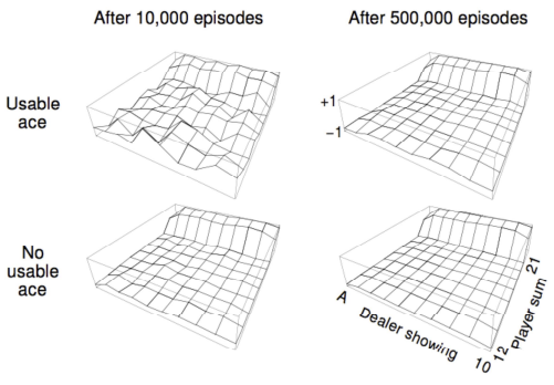
Look at the blackjack example in the slides
Temporal-Difference learning
The goal of TD learning is to learn the state-value function online and incrementally. TD improves upon Monte-Carlo methods through two key mechanisms:
- Step-by-step Updates: The value function is updated after every interaction, rather than waiting for the episode’s conclusion.
- Bootstrapping: The agent updates its current value estimate using its own estimate of the next state’s value.
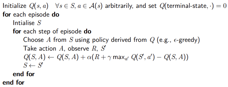
THE TD(0) ALGORITHM
TD(0) is the simplest form of temporal-difference learning. It updates the value toward a TD Target, which consists of the immediate reward plus the discounted value of the next state .
Therefore the update rule is:
where:
- TD Target : is the estimated total return from the perspective of the next time step.
- TD Error : The difference between the TD Target and the current estimate .
At the start of the learning process, value estimates ( and ) are inaccurate. However, each update combines a certain reward (real feedback) with an uncertain estimate (the next state’s value). Because the reward is a ground-truth signal, each update incrementally pulls the value function toward reality. Over time, these improved estimates propagate backward through the state space, making the entire value function increasingly reliable.
MC VS. TD
The fundamental difference between Monte-Carlo (MC) and Temporal-Difference (TD) learning lies in when and how they update their knowledge:
- TD is “Online”: it updates the value function after every step. If an episode lasts steps, TD performs updates, enabling continuous and incremental learning.
- MC is “Offline”: It must wait until the end of an episode to observe the total return before performing a single update.
In practice: For long episodes, an MC agent stays “blind” to its performance until the very end, while a TD agent adjusts its behavior continuously.
Another key difference concerns sequence requirements:
- TD handles incomplete sequences: it can learn from partial interactions without knowing the final outcome. This is useful in tasks with long horizons where reaching the end is rare or time-consuming.
- MC requires complete sequences: because it relies on the actual total return, learning can occur only after the episode terminates.
As a result, TD can operate in continuing (non-terminating) environments, while MC is limited to episodic (terminating) environments.
BIAS/VARIANCE TRADE-OFF
In reinforcement learning, the choice between Monte Carlo (MC) and Temporal Difference (TD) methods reflects a trade-off between bias and variance.
- The Return is an unbiased estimate of the true value because it reflects the actual rewards observed until the end of the episode.
- The TD Target is a biased estimate of because it relies on the agent’s current estimate of the next state value rather than the true value.
- The True TD target would be an unbiased estimate of , but the true value function is unknown.
Comparison of Performance:
-
Temporal Difference (Low Variance, High Bias): The TD target depends on only a single transition (one action, one reward, and the resulting state). Because fewer random variables are involved in each update, it has much lower variance. Although bootstrapping introduces bias, the reduced noise allows the agent to learn faster.
-
Monte Carlo (High Variance, Zero Bias):
While MC is unbiased, it relies on the final return, which is the sum of many actions, transitions, and rewards. This accumulation of random events leads to high variance, requiring a large number of episodes to obtain accurate estimates.
In practice, it is often preferable to accept a slightly biased estimate if it can be obtained more efficiently. This reflects a common situation in optimization, where approximate solutions are preferred over exact ones because they are computationally feasible and faster to compute.
Model-free control
- Model-free prediction focuses on estimating the value function for a given policy when the environment model is unknown.
- Model-free control instead focuses on finding a good policy without knowledge of the environment model.
Common approaches to model-free control include:
- On-Policy Monte Carlo Control
- On-Policy Temporal-Difference Learning
- Off-Policy Learning
IMPROVING A POLICY
Given a policy the general approach is:
- Policy Evaluation: the agent evaluates the current policy by estimating its value functions:
- Policy Improvement: the agent uses these value estimates to build a better policy.
A common method is to act greedily with respect to the current estimates:
In model-free contexts, we must rely on the action-value function for policy improvement. Being greedy with respect to the state-value function requires a model of the environment to know which action leads to which state (transition probabilities). Without a model, only directly tells the agent which action yields the highest expected return from the current state.
THE EXPLORATION DILEMMA
A greedy policy always selects the action that maximizes the current estimated return.
If an agent is in front of a door and evaluates that moving “Left” yields a reward of 0 while moving “Right” yields a reward of 1, a greedy policy will always choose “Right” from that point forward.
While acting greedily maximizes immediate performance based on current knowledge (exploitation), it has a significant flaw: it does not explore. If the agent only selects the action with the highest current estimate:
- It never tests alternative actions.
- It may miss superior actions that haven’t been explored yet.
This creates the fundamental Exploration vs. Exploitation dilemma: the agent must balance choosing what it knows to be good with trying new things to discover what might be better.
-GREEDY EXPLORATION
The -greedy policy is a standard solution to the exploration-exploitation dilemma. It ensures that all available actions are sampled with a non-zero probability, preventing the agent from prematurely converging on a suboptimal strategy.
At each decision point the agent:
- With probability choose the “greedy” action, the one with the highest current value estimate.
- With probability select an action at random from all possible options (including the greedy one).
ON AND OFF POLICY LEARNING
Another important distinction in reinforcement learning is between:
- On-policy: the agent evaluates and improves the exact policy it is currently using to interact with the environment. Learn about policy using experience sampled directly from .
Person learns that a specific move is dangerous because they attempt it themselves and experience the immediate consequence.
- Off-Policy: The agent learns about a target policy while following a different behavior policy that could be more exploratory.
An athlete observes how a professional moves, extracts useful dynamics from those observations, and then applies that knowledge to their own performance
Off-policy learning is often advantageous because it allows the agent to reuse experience generated by old policies , even if those policies are not optimal.
Monte-Carlo Control
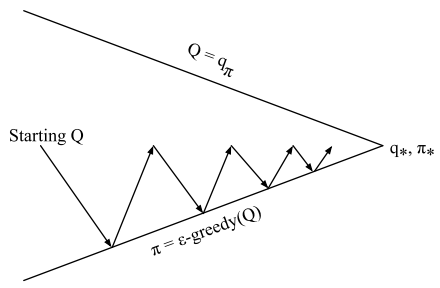
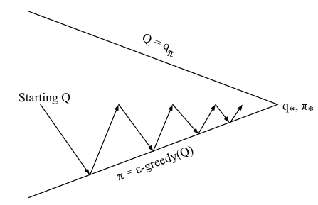
MONTE-CARLO POLICY ITERATION
In Monte Carlo (MC) control, the agent seeks the optimal policy by alternating between two fundamental phases:
- Policy evaluation: The agent estimates the action-value function () for the current policy . This is typically initialized to zero, representing a lack of prior knowledge.
- Policy improvement: The agent refines its behavior using an -greedy policy based on the current estimates.
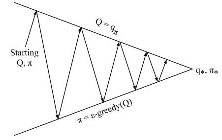
By repeatedly cycling through evaluation and improvement, the agent’s behavior and value estimates gradually converge toward the optimal action-value function () and the optimal policy ().
ON-POLICY MONTE-CARLO CONTROL
A practical and efficient implementation of this cycle is On-Policy MC Control. While traditional policy iteration theoretically requires the evaluation phase to fully converge (infinite episodes) before improving the policy, this is inefficient in practice.
Instead of waiting for full convergence, we perform incomplete evaluation. The agent updates the value function and improves the policy simultaneously after every single episode.
The term “On-Policy” specifically means the agent is evaluating and improving the same policy it uses to make decisions.
TD control
Temporal-Difference (TD) learning offers several advantages over Monte-Carlo (MC) methods, including lower variance and the ability to learn online from incomplete sequences.
By applying these TD principles to the control loop, we can estimate the action-value function and improve the policy at every time-step using -greedy selection.
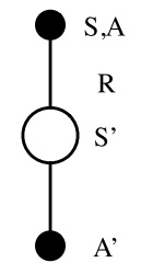
SARSA
SARSA is a primary TD control algorithm named after the sequence of variables it processes:
The agent updates its action-value estimate using the following TD update rule:
ON-POLICY CONTROL WITH SARSA
SARSA is an on-policy algorithm. This means the action used to calculate the TD target in the update rule is selected using the same policy () that the agent uses to interact with the environment.
Every time-step:
- Policy evaluation with Sarsa, the agent updates to better approximate →
- Policy improvement with -greedy policy improvement.
Algorithm
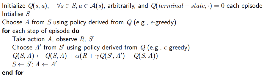
-
Initialization
The agent initializes the Q-table for every state-action pair, with zero-values representing a lack of prior knowledge.
-
Interaction Loop
For each step of an episode, the agent follows this sequence:
- Initial State & Action: The agent observes the current state and selects an action using its -greedy policy.
- Execution: The agent executes action , receiving a reward and transitioning to a new state
- Next Action Selection: From the new state , the agent selects the next action using the same -greedy policy.
- Update: The agent uses to update the value of the previous state-action pair .
- Transition: The agent sets and , repeating the process until a terminal state is reached.
Example of Windy gridworld
Q-learning
Q-learning is the most prominent off-policy Temporal Difference (TD) control algorithm. It allows an agent to evaluate and improve a target policy while following a different behavior policy .
By decoupling the learning process from the behavior, Q-learning enables several powerful techniques:
- Imitation Learning: Learning by observing a human or another agent.
- Experience Replay: Reusing data generated by previous policies.
- Safe Exploration: Converging on a purely greedy optimal policy while using a highly exploratory behavior policy to navigate the environment.
THE UPDATE RULE
The fundamental difference between SARSA and Q-learning lies in how the next action is used in the update:
- In SARSA, the update uses the action actually chosen by the behavior policy.
- In Q-learning, the update assumes the agent will take the best possible action in the next state, regardless of what the behavior policy actually chooses.
During training, the agent selects the next action using the behavior policy , but the update is performed as if the agent followed the target policy . The Q-value of the current state–action pair is therefore updated toward the value of a successor action chosen according to the target policy :
OFF-POLICY CONTROL WITH Q-LEARNING
In off-policy Q-learning, both the behavior policy and the target policy are allowed to improve over time:
- The target policy is defined as greedy with respect to the current Q-values:
- The behavior policy remains exploratory (e.g., -greedy), to ensure sufficient exploration.
Because the target policy is greedy, the Q-learning target simplifies:
ALGORITHM
-
Initialization
The Q-table is initialized for all state-action pairs (typically to 0), and the terminal state is set to 0.
-
Interaction and Learning
- Starting from a state , the agent selects an action using the -greedy behavior policy .
- The agent then observes:
- The immediate reward
- The next state
- At each step, the -value is updated as:
- The agent moves to the new state and repeats the process until the end of the episode.
Theoretical guarantee: if every state–action pair is visited infinitely often and the learning rate decays appropriately, Q-learning converges to the optimal action-value function:
Value Function Approximation
So far, we have represented value functions using lookup tables, where:
- Every state has an entry
- Every state-action pair has an entry
While this approach is effective for simple environments, it becomes impractical for complex problems. In environments with high-dimensional or continuous state spaces, there are too many states/or actions to store in memory, and learning each value individually becomes too slow.
Solution:
Instead of storing every value explicitly, we learn a parameterized function that approximates the value using a set of weights:
This approach allows the agent to generalize its knowledge from seen states to unseen states.
Rather than updating a single table entry, we update the parameter vector using standard reinforcement learning methods like Monte Carlo (MC) or Temporal Difference (TD) learning.
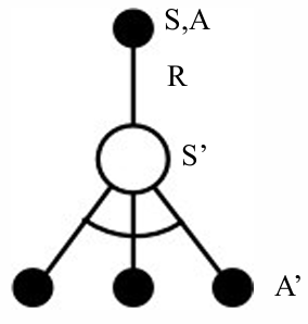
TYPES OF VALUE FUNCTION APPROXIMATION
There are many possible function approximators, for example:
- Linear combinations of features
- Neural network
- Decision tree
- Nearest neighbour
- Fourier / wavelet bases
- …
In reinforcement learning, the training method must be suitable for non-stationary and non-iid data, since the data distribution changes as the agent interacts with the environment and updates its policy.
Incremental Methods
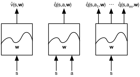
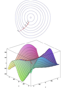
GRADIENT DESCENT
If is a differentiable function of a parameter vector , its gradient represents the direction of the steepest increase:
To find a local minimum of , we adjust in the direction of the negative gradient. The update rule is defined as:
where is a step-size (learning rate) parameter.
VALUE FUNCTION APPROXIMATION BY SGD
In Reinforcement Learning, the goal is to find a parameter vector that minimizes the Mean-Squared Error (MSE) between the approximate value function and the true value function :
Using gradient descent to find a local minimum results in the following update:
Stochastic Gradient Descent (SGD) simplifies this by sampling the gradient at each step rather than calculating the full expectation. The expected update remains equal to the full gradient update:
FEATURE VECTORS
To apply function approximation effectively, we represent a state as a feature vector :
Examples of Features
- Robotics: Distances from specific landmarks.
- Finance: Moving averages or trends in the stock market.
- Games (Chess): Specific configurations of pieces and pawns.
A well-designed feature vector acts as the bridge between perception and decision-making. It is fundamental for:
- Efficiency: Avoiding redundant or inefficient state representations.
- Dimensionality Reduction: Compressing a vast state space into a manageable set of inputs.
- Generalization: Allowing the agent to estimate the value of states it has never seen by identifying similar features.
Feature representations allow the model to capture relevant structure in the environment, avoiding the need to encode every possible state explicitly. Without accurate feature encoding, an agent cannot reliably learn the value of its states or actions in complex environments.
Linear value function approximation
In linear function approximation, the value function is represented as a linear combination of features. Given a feature vector and a weight vector , the approximate value is defined as:
The objective function is quadratic in terms of the parameters :
Because the objective is quadratic, Stochastic Gradient Descent (SGD) is guaranteed to converge to the global optimum. The gradient is simply the feature vector itself, , leading to a highly efficient update rule:
This formula states that the update is the product of:
Update = stepsize prediction error feature value
Structurally, this model can be viewed as a single-layer neural network without an activation function.
TABLE LOOKUP FEATURES
Interestingly, traditional tabular reinforcement learning (like Q-learning and SARSA) is a special case of linear approximation. This occurs when we use Table Lookup Features, where the state space is represented by a “one-hot” encoded vector.
For a state space with states, the feature vector contains a at the index corresponding to the current state and elsewhere:
In this specific case, the parameter vector directly provides the value of each individual state:
Incremental prediction algorithms
In supervised learning, we assume a supervisor provides the true value . In reinforcement learning, we must substitute this missing supervisor with a target derived from experience:
- For Monte Carlo (MC): the target is the actual return :
- For TD(0): the target is the TD target :
MONTE-CARLO WITH VALUE FUNCTION APPROXIMATION
The return is an unbiased but noisy sample of the true value . This allows us to treat the episode data as a supervised training set:
Linear MC Policy Evaluation:
When using linear approximation, the update simplifies using the feature vector :
Procedure & Properties:
- Storage: Record all states visited during an episode.
- Calculation: At the episode’s end, compute the total return for each state.
- Update: Use the (state, return) pairs as training data to update weights.
MC evaluation converges to a local optimum, even with non-linear function approximators (like neural networks). However, the primary drawback remains that updates can only occur after an episode terminates.
TD WITH VALUE FUNCTION APPROXIMATION
The TD target serves as a biased sample of the true value . We generate training data by pairing the current state with a target composed of the immediate reward and the estimated value of the successor state:
The update uses the TD error () and the feature vector :
Advantages & Convergence:
- Online Learning: Updates are performed at every step, allowing the agent to learn during the episode without waiting for termination.
- Convergence: Linear TD(0) is mathematically guaranteed to converge near the global optimum.
Action-value function approximation
The principles used for state-value approximation extend directly to the action-value function. The goal is to approximate using a parameterized function that accounts for both the current state and the action taken.
Objective Function
We aim to minimize the Mean-Squared Error (MSE) between the approximate action-value function and the true action-value function :
To find a local minimum, we apply SGD. The weight update is proportional to the prediction error and the gradient of the approximation function:
The learning procedure is identical to the state-value approach, with the input space extended to incorporate the action.
LINEAR ACTION-VALUE FUNCTION APPROXIMATION
In the linear case, the relationship between features and values is straightforward. The state-action pair is represented by a feature vector:
The action-value function is the dot product of the feature vector and the parameter vector:
Since the gradient of a linear function is simply the feature vector itself, , the update rule becomes:
Incremental control algorithms
As in prediction methods, we replace the unknown value with a target:
- For Monte Carlo (MC), the target is the return :
- For TD(0) (SARSA), the target is the TD target :
These updates adjust the parameter vector incrementally to reduce the difference between the predicted value and the chosen target.
Convergence of prediction algorithms
Convergence guarantees vary significantly depending on the representation (Tabular, Linear, or Non-Linear) and the learning approach (On-Policy vs. Off-Policy).
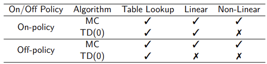
Key Takeaways
- Monte Carlo (MC) prediction is theoretically robust. It converges under standard assumptions regardless of whether a tabular, linear, or non-linear (e.g., neural network) representation is used. This stability applies to both on-policy and off-policy learning.
- Temporal-Difference (TD) methods have weaker theoretical guarantees. While convergence is guaranteed in the tabular case, it is not always mathematically guaranteed when using linear or non-linear function approximation.
Despite this limitation, TD methods are widely used in practice because they learn significantly faster than Monte Carlo methods. Convergence is generally achieved by using a sufficiently small learning rate.
Monte Carlo methods, although theoretically sound, can be extremely slow, making them impractical for many real-world problems.
Convergence of control algorithms
Control algorithms—where the policy is updated alongside the value function—face even stricter challenges, particularly with function approximation.
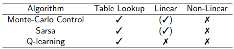
Note on “Chattering”: In linear cases, the value function may not settle on a single point but will “chatter” (oscillate) around a near-optimal solution.
Batch Methods
While standard Gradient Descent is simple, it is often sample inefficient because it processes each experience once and then discards it. Batch methods address this by seeking the best-fitting value function based on the agent’s entire history of experience (“training data”).
LEAST SQUARES PREDICTION
Given a value function approximation and a dataset of experience containing pairs:
The goal is to find the parameter vector that minimizes the Sum-Squared Error (LS) between the approximate values and the target values across the entire dataset:
STOCHASTIC GRADIENT DESCENT WITH EXPERIENCE REPLAY
Experience Replay is a practical implementation of batch reinforcement learning. Instead of performing a single update per transition, the agent stores its experiences and repeatedly samples from them to train the model.
The Process
Given the experience dataset :
- Sample: randomly select a pair from the history:
- Update: apply the stochastic gradient descent (SGD) update:
- Repeat: iterate this process multiple times until it converges to the least-squares solution:
Experience replay in deep Q-networks (DQN)
DQN combines Q-learning with deep neural networks. Using non-linear function approximators with TD learning can be unstable, so DQN introduces two key stabilization techniques:
- Experience Replay
- Fixed Q-Targets.
Two neural networks are used:
- A learnable network, updated via gradient descent
- A frozen (target) network, providing stable Q-value targets
The Learning Loop:
- Action Selection: The agent selects an action using an -greedy policy based on the current network weights.
- Storage: The resulting transition is stored in a Replay Memory ().
- Sampling: Instead of learning only from the most recent step, the agent samples a random mini-batch of transitions from . This breaks the temporal correlation between consecutive samples.
- Target Calculation: The agent computes the Q-learning targets using a separate set of old, fixed parameters (). This “Target Network” prevents the target from moving too quickly, which stabilizes the update.
- Optimization: the agent minimizes the Mean-Squared Error (MSE) loss function using a variant of Stochastic Gradient Descent:
After each parameter update, a new loss is computed using the latest mini-batch, and the agent may select new actions accordingly. Convergence occurs when Q-values stabilize.
DQN is off-policy because it uses a Behavior Policy (-greedy) to collect experiences into a buffer, but it updates its knowledge based on a Target Policy (purely greedy ). Since the data being used for training can come from any previous policy stored in the Replay Buffer, the agent is effectively learning the optimal strategy by ‘observing’ its own past mistakes and successes.
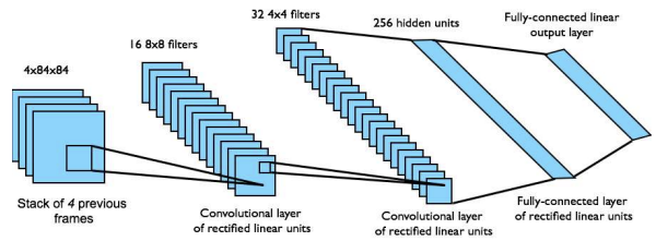
DQN IN ATARI
DQN is a model-free, off-policy reinforcement learning algorithm that learns the action-value function end-to-end directly from raw pixels, without the need for hand-engineered features.
It was used in Atari games:
- To provide the agent with a sense of motion and temporal context (such as the speed and direction of a ball), the input state is not a single image. Instead, it is a stack of raw pixels from the four most recent frames.
- The input stack is processed through a Convolutional Neural Network (CNN) that automatically extracts spatial features (like the positions of paddles or enemies):
- Output Layer: The final layer is a fully connected layer with 18 outputs, each corresponding to a specific joystick/button configuration.
- Q-values: Each output represents the estimated for that action, allowing the agent to select the one with the highest expected return.
- Reward: defined as the change in game score at each step.
Key Takeaways
| Concept | Description |
|---|---|
| Reinforcement Learning | Agent learns by interacting with an environment to maximize cumulative reward — no labels, delayed feedback, sequential non-IID data |
| Agent–environment loop | At each step : observe , receive reward , take action → environment transitions and emits |
| Policy | Deterministic or stochastic — defines agent behavior |
| Return | Discounted cumulative reward ; trades off myopic vs far-sighted |
| State / action value | ; |
| Bellman expectation | ; analogous form for — recursive decomposition |
| Model | Internal representation: for transitions, for rewards. Enables planning |
| Model-free prediction | Estimate directly from experience without knowing the environment dynamics |
| Monte Carlo (MC) | Average actual returns over episodes; unbiased, high variance, requires terminating episodes |
| TD(0) | . Online, biased, low variance |
| MC vs TD | MC: unbiased, slow, episodic only. TD: biased (bootstraps), fast, works with incomplete sequences |
| Bias–variance trade-off | MC return = unbiased high-variance; TD target = biased low-variance — TD usually wins in practice |
| Generalized Policy Iteration | Alternate policy evaluation ( or ) with policy improvement (greedy w.r.t. estimates) |
| -greedy | With prob. pick the greedy action; with prob. pick uniformly — guarantees exploration |
| On-policy vs off-policy | On-policy: learn the policy you use to act. Off-policy: learn target policy while behaving with |
| SARSA | On-policy TD control: with from the same policy |
| Q-learning | Off-policy TD control: target uses regardless of behavior policy → converges to |
| Function approximation | Replace tabular with parameterized — needed for large/continuous state spaces |
| Linear approximation | . Quadratic objective → SGD reaches global optimum; gradient = feature vector |
| Convergence | Tabular: always converges. Linear on-policy: usually OK. Non-linear / off-policy: no guarantees |
| Experience replay | Store transitions in a buffer, sample mini-batches → breaks temporal correlation, reuses experience |
| DQN | Q-learning + deep CNN + replay buffer + fixed target network ( updated periodically). Plays Atari from raw pixels |
| Why DQN is off-policy | Behavior policy is -greedy, target policy is greedy (), and stale buffer data is replayed |