Graph Neural Networks
CONVOLUTIONAL NEURAL NETWORKS
Convolutional Neural Networks (CNNs) are a class of deep neural networks particularly effective for processing grid-structured data, such as images.
They use filters (kernels) stacked in successive layers to increase depth and promote a hierarchical extraction of features.
Up to now, we have seen that the 2D spatial cross-correlation between an input image and a square kernel is defined as:
Where:
-
is the kernel size (square)
e.g.
-
: input pixel
-
: kernel weight
THE EUCLIDEAN LATTICE ASSUMPTION
From a geometric point of view, the input image can be seen as a regular 2D grid of values. Conceptually, each pixel exists on a discrete 2D lattice (e.g., ), which can be viewed as a 2D Euclidean plane.
A discrete lattice is a regular grid of points in Euclidean space where each point has integer coordinates, and the distance between neighboring points is fixed.
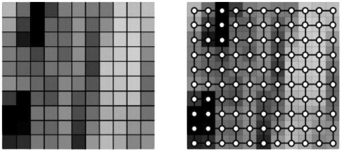
Having such a regular and predictable structure is important because it allows the kernel to slide uniformly over the image, applying the same operation everywhere.
The cross-correlation operation slides a kernel across this grid, systematically visiting each location. So at each position, the kernel interacts with a local patch of the input. This means the operation captures local relationships — how each pixel relates to its immediate neighbors in that 2D space.
Note: Although the operation is discrete, the grid itself can be viewed as a sampling of a continuous 2D Euclidean domain.
CROSS-CORRELATION 1D ON A 1D EUCLIDEAN LATTICE
Just like in 2D, the 1D grid can be seen as a discretization of a continuous Euclidean line , sampled at regular intervals.
Both the input signal and the kernel are defined on a 1D Euclidean lattice, and the kernel slides along this lattice, computing local interactions at each position.
A GRAPH-BASED PERSPECTIVE
Under this new viewpoint, the input image can be seen as a signal defined on a (Euclidean) graph.
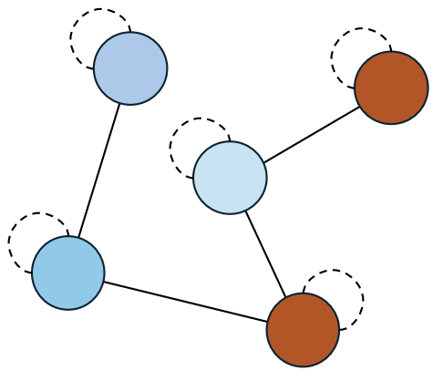
A graph consists of:
- A set of nodes (vertices)
- A set of edges
Graphs can be:
- Directed or undirected
- Weighted or unweighted
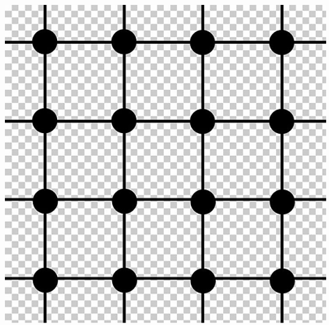
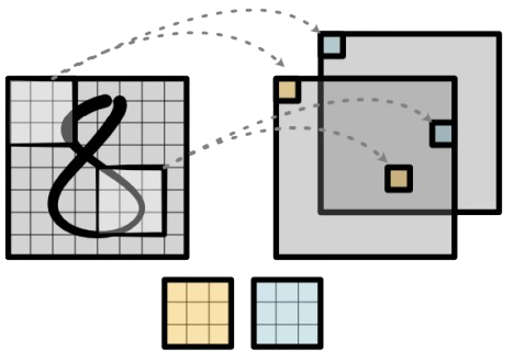
A graph is defined as a lattice graph when its nodes are arranged on a regular grid (e.g., 1D, 2D, or 3D). In this model, we can map the image structure as follows:
- Each pixel corresponds to a node in the graph.
- Each node is associated with a feature vector (e.g., a triplet of raw RGB values).
- The edge set connects each node to its spatial neighbors using a fixed connectivity rule (e.g., 4-connected: top, bottom, left, right).
PROBLEM OF STANDARD N-D CONVOLUTION
Traditional convolutional architectures assume data is defined over regular Euclidean grids (e.g., 1D signals, 2D images).
However, not all types of data exhibit this regular structure. Many real-world domains — such as:
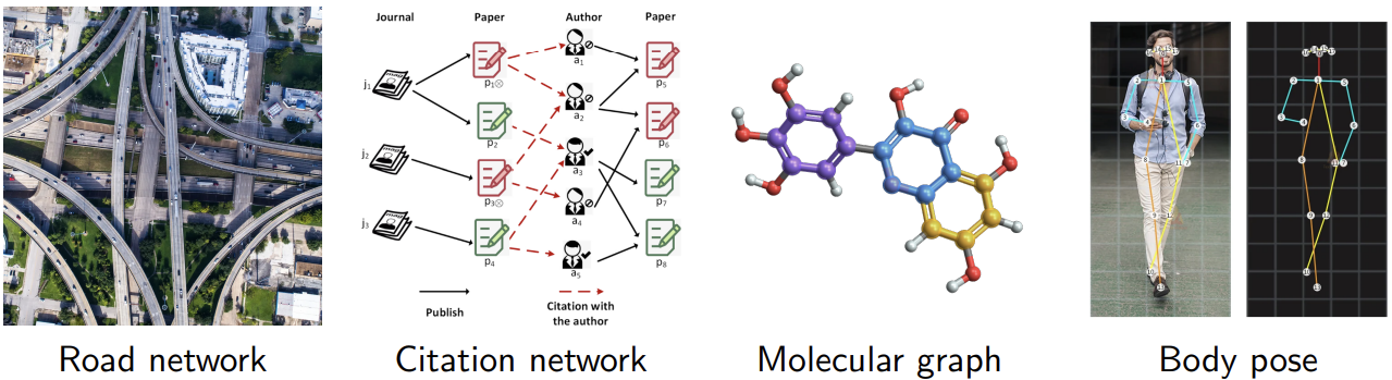
are non-Euclidean.
In these domains, entities (or nodes) have irregular connections: some nodes are highly connected while others are not, and the relationships among nodes do not follow a fixed grid.
Graph Neural Network (GNN)
OBJECTIVE
The objective is to define a neural network that can handle graph-structured data.
The main challenges in a Graph Neural Network (GNN) are:
- Irregular structure: nodes may have different numbers of neighbors, meaning there is no fixed-size receptive field.
- No spatial locality: unlike images, there is no inherent notion of distance or order between nodes.
- Permutation invariance: the output should not depend on the order in which nodes are processed.
- No global coordinate system: there is no fixed layout or orientation to rely on.
- Dynamic topology: edge connectivity may evolve over time or depend on node features.
GRAPH CONVOLUTIONAL NETWORKS
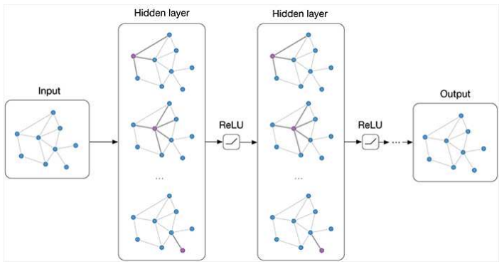
Graph Convolutional Networks (GCNs) generalize the concept of convolution to graph-structured data. As with standard neural networks:
- A Graph Neural Network is composed of multiple successive layers.
- It includes input features, hidden activations (often called node embeddings), activation functions, and output responses.
- Gradient descent and backpropagation are used to update the model parameters.
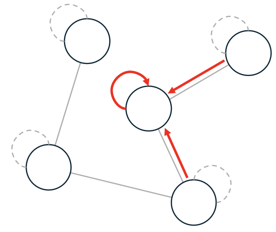
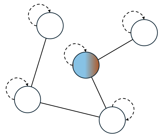
The key idea in GCNs is message passing, meaning that the information is propagated across the graph by allowing each node to communicate with its neighbors.
In practice, this means that each node updates its state by aggregating information from its neighbors and updating its own representation accordingly. So we have two main steps:
-
Aggregation (Leveraging the graph structure)
Each node aggregates information from its neighbors by combining their embeddings using an aggregation function (e.g., sum, mean, max, or a learned function).
-
Node update
The aggregated information is then passed through a neural network layer (e.g., a simple MLP) to generate a new node representation (embedding).
This updated embedding captures both the node’s own features and those of its local neighborhood.
This process can be stacked across multiple layers, enabling nodes to gradually capture information from larger neighborhoods.
AN EXAMPLE: GCN
GCN Layer represents one of the most prominent examples of graph-based neural networks.
It takes in input:
- Node features matrix where each row corresponds to the feature vector of a node.
- Adjacency matrix which encodes the graph structure — which nodes are connected. It can be:
- binary
- weighted.
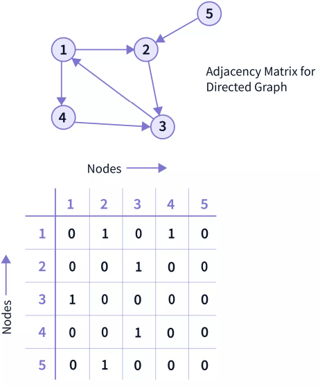
In a simple, unweighted graph, if node i and node j are connected, then ; otherwise,
THE ROLE OF THE ADJACENCY MATRIX
The adjacency matrix is a key component of GNNs:
-
Acts as a structural prior
The adjacency matrix encodes geometric or relational constraints of the domain.
-
Enables the model to reflect spatial or structural constraints of the data.
-
Helps reduce overfitting by:
- Enforcing locality, meaning that each node only aggregates from its true neighbors.
- It introduces an inductive bias, built-in assumptions about how the data is structured, which helps the model generalize better on unseen data.
The adjacency matrix is typically derived from domain knowledge — it is fixed manually and remains constant across layers. In contrast, the node features (embeddings) are updated layer by layer through the message-passing mechanism.
When the structure is not known, the adjacency matrix can be constructed automatically using heuristic methods, such as -nearest neighbors in feature space or distance thresholds.
MESSAGE PASSING
Layer-wise propagation rule:
- → adjacency matrix with self-loops added
- → symmetric normalization of the adjacency matrix
- with is the (diagonal) degree matrix
- → node embeddings from the previous layer
- → learnable weight matrix (projection)
- → activation function (e.g., ReLU)
PROJECTION
The same operation can be expressed more intuitively in a node-wise (local) form:
-
Aggregation:
Each node collects (aggregates) features from its neighbors and from itself, weighting each contribution by the inverse of the node degrees. This keeps the aggregation balanced regardless of how many neighbors each node has.
-
Projection:
The aggregated message is then transformed (linearly projected) into a new feature space through the learnable weights .
-
Non-linearity:
Finally, a non-linear activation (e.g., ReLU) is applied to obtain the updated embedding of node
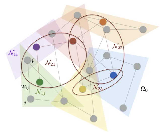
RECEPTIVE FIELD AND THEORETICAL MOTIVATIONS
A GCN layer aggregates information from each node’s immediate (1-hop) neighbors. Stacking multiple layers allows the model to capture information from higher-order neighborhoods:
- 1 layer → information from direct neighbors (1-hop)
- 2 layers → information from neighbors of neighbors (2-hop)
- …
- k layers → information from the k-hop neighborhood
This defines the receptive field of each node — the portion of the graph that influence a node’s representation.
The full two-layer GCN can be written as:
The GCN can be theoretically motivated by spectral graph theory:
- It represents a first-order approximation of spectral graph convolutions.
- Based on the spectral formulation of convolution on graphs.
Applications of GNNs
Node Classification
In node classification, the goal is to predict a label for each node in the graph. Every node is associated with an input feature vector , which encodes its attributes or properties.
The model processes these features through multiple GNN layers, allowing each node to aggregate information from its neighbors and produce a node embedding .
A final classification layer then maps these embeddings to class scores:
The predicted label for each node is obtained by taking the class with the highest score:
The overall model output is a matrix:
where:
- is the number of nodes in the graph and each row corresponds to a node’s class scores.
- is the number of possible classes.
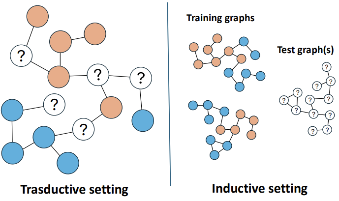
TWO SETTINGS
- Transductive setting, the entire graph is available during training, but only a subset of nodes has known labels. The main objective is to predict the labels of the remaining nodes within the same graph. Since the full structure is accessible, the model can take advantage of the connections among all nodes — both labeled and unlabeled. Even though the unlabeled nodes are not directly supervised, they still contribute to the learning process by sharing structural information that helps the model understand the overall graph context.
- Inductive setting requires the model to generalize to completely new nodes or even entirely unseen graphs. These nodes are not part of the training data, so the model cannot rely on their connections during learning. Instead, it must base its predictions on the available node features and their local neighborhood structure. The goal is for the model to learn representations that can effectively transfer across different graphs and remain useful in new, unseen scenarios.
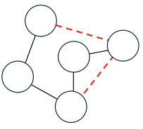
Link Prediction
In link prediction, the task is to predict whether a link (or edge) exists between two nodes in a graph. Given a pair of nodes and , the goal is to predict if .
This is typically formulated as a binary classification problem on node pairs, although it can also become a multi-class problem when different edge types are considered.
A common pipeline involves three main steps:
- Learning node embeddings and using a GNN.
- Computing an edge representation →
- Mapping this representation to class scores with a linear layer
- Prediction step
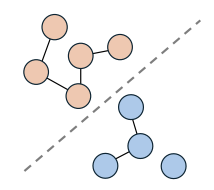
Graph Classification
In graph classification, the goal is to assign a label to an entire graph rather than to individual nodes or edges.
Each graph is treated as a single data point. Node features are first processed by several GNN layers to obtain node embeddings , which are then aggregated into a single graph-level vector through a global pooling operation:
Finally, a multi-layer perceptron (MLP) is used to predict the label for the entire graph:
Problem
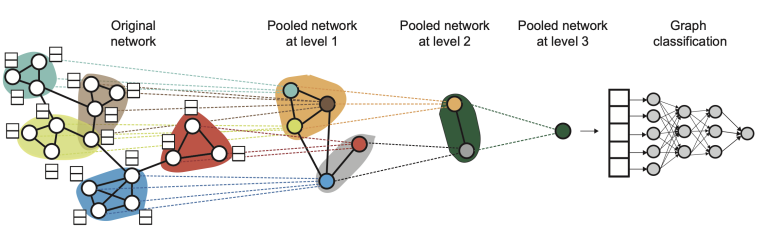
In Graph Neural Networks (GNNs), the graph convolutional layers do not change the number of nodes in the graph. After several convolutional layers, we still obtain a representation for each individual node, but not a single, unified representation for the entire graph.
This poses a problem when we want to perform graph-level predictions, such as classifying an entire graph rather than its individual nodes. In such cases, we need a mechanism to aggregate information from all nodes into one compact vector that represents the whole graph.
Solution: Global Pooling
The Global Pooling mechanism addresses this issue by aggregating the embeddings of all nodes into a single global representation. This operation effectively creates a “super-node” that summarizes the structural and feature information of the entire graph.
Common global pooling methods include:
- Global average pooling:
- Attention-based pooling:
While these methods summarize all node embeddings in a single step, other approaches introduce hierarchical pooling, similar to what convolutional neural networks (CNNs) do in image processing.
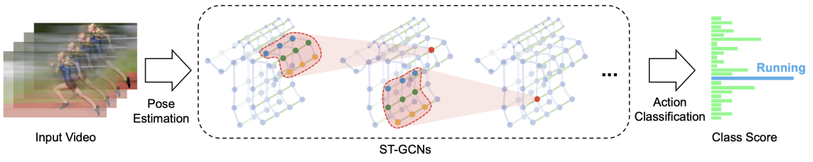
EXAMPLE
A common application of graph classification is action recognition from human skeleton data. Here, each sequence of human poses is represented as a spatio-temporal graph, where:
- Spatial edges connect body joints within each frame.
- Temporal edges connect the same joint across consecutive frames.
By applying Graph Neural Networks (GNNs) or Spatio-Temporal Graph Convolutional Networks (ST-GCNs), it becomes possible to jointly model both spatial and temporal relationships, enabling accurate classification of the performed action.
Graph Attention Networks (GAT)
PROBLEMS OF GCN
The layer-wise propagation rule of a Graph Convolutional Network (GCN) is defined as:
Although this formulation enables effective message passing across graph nodes, standard GCNs suffer from several limitations:
- Over-smoothing: As the number of layers increases, node representations from different parts of the graph become indistinguishable making it difficult to separate nodes by class or role.
- Aggregation: In each layer, every neighboring node contributes equally to the target node’s update. This lack of adaptive weighting or attention ignores the fact that some neighbors may be more informative or relevant than others.
- Limited expressivity: The model’s capacity to capture complex relationships is constrained by the relations encoded in the adjacency matrix.
GRAPH ATTENTION NETWORKS (GATs)
Graph Attention Networks (GATs) extend traditional Graph Convolutional Networks (GCNs) by integrating an attention mechanism that enables nodes to assign different levels of importance to their neighbors during message passing.
Key concepts:
-
Learned edge weights:
Unlike GCNs, GATs do not rely on a pre-defined weighted adjacency matrix. Instead, they learn attention coefficients that determine how much influence each neighbor should have.
-
Local adaptivity:
Different neighbors receive different weights, allowing the model to focus more on relevant nodes.
In essence, through the attention mechanism, each node attends to its local neighborhood, using the adjacency matrix as a structural guide.
This is done in five steps:
-
Linear Projection
Each node’s feature vector is first linearly transformed:
where:
- is a learnable weight matrix shared across all nodes.
-
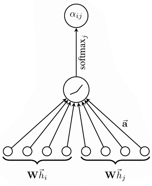
Attention Coefficients:
For every edge , the model computes an unnormalized attention score between node and its neighbor :
where:
- denotes vector concatenation.
- is a learnable weight vector.
The affinity score indicates the importance of node ’s features to node .
In the most general case, the model allow all nodes to attend to every other node, dropping all structural information. However, to maintain locality, GATs introduce masked attention, which restricts attention to first-order neighbors:
where is the first-order neighbors of (including ) expressed in the adjacency matrix.
Advantage. The graph is not required to be undirected; the computation of the attention coefficient can be simply omitted if the edge is not present.
-
Normalization:
The unnormalized attention coefficients are converted into normalized attention scores across all neighbors of :
-
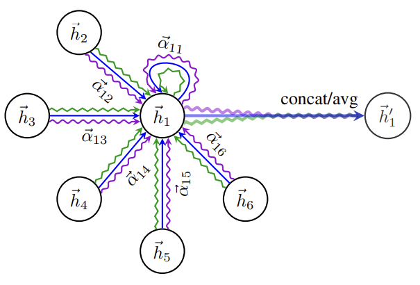
Aggregation
The final node representation is obtained by taking a weighted sum of the transformed features of its neighbors:
-
Multi-head Attention
To stabilize learning and enhance expressivity, GATs often employ multi-head attention. In this case independent attention mechanisms are applied, and their outputs are concatenated:
Note that, in this setting, the final returned output, , will consist of features (rather than ) for each node.
GATs can also be combined with residual connections to improve gradient flow and stabilize deeper architectures.
COMPARISON: GAT VS SELF-ATTENTION
| Aspect | GAT | Self-Attention (Transformers) |
|---|---|---|
| Input structure | Graph (nodes + edges) | Sequence (e.g., tokens) |
| Neighborhood | Defined by adjacency matrix | Full attention (every token attends to all others) |
| Sparsity | Sparse: only local neighbors | Dense: full pairwise interactions |
| Attention mechanism | Single-layer MLP over concatenated node pairs | Dot-product between learned query and key vectors |
| Position encoding | Implicit via graph topology | Explicit (e.g., sinusoidal or learned) |
| Inductive bias | Local, relational inductive bias from graph edges | Temporal or spatial bias via positional encodings |
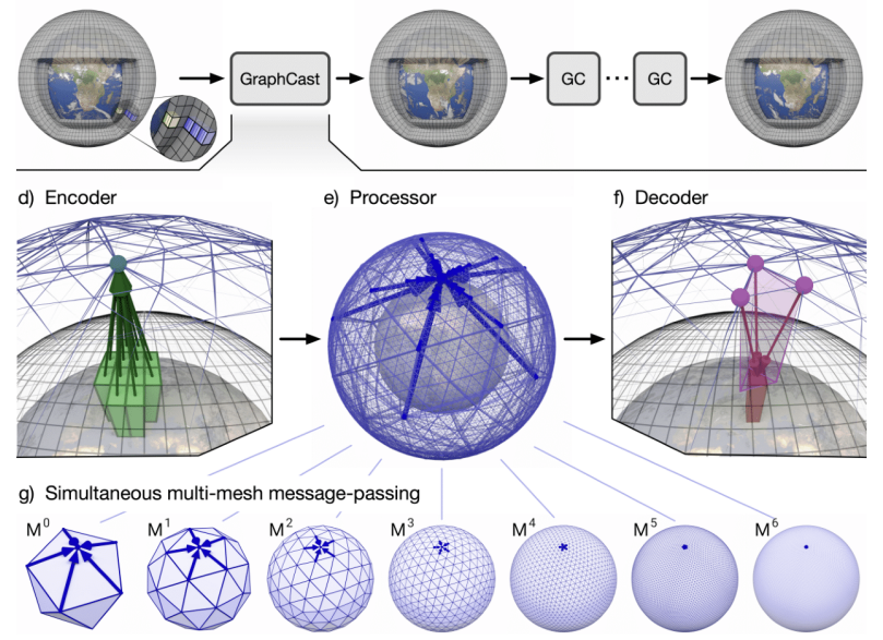
GraphCast
WEATHER FORECASTING WITH GNNs
GraphCast is a state-of-the-art model for medium-range weather prediction that uses Graph Neural Networks to model the Earth’s atmosphere:
- Nodes: grid points on a spherical mesh (icosahedral grid)
- Edges: connect spatially adjacent locations, representing local interactions in the atmosphere
- Node features: meteorological variables such as wind, temperature, pressure, humidity, etc.
Performance:
- For 10-day forecasts, GraphCast achieves accuracy comparable to traditional physics-based systems like HRES, the leading deterministic operational forecast model.
- Offers significantly faster inference, enabling rapid predictions across the globe.
ARCHITECTURE
GraphCast combines temporal sequence modeling with GNN-based message passing:
- Message-passing GNN layers are used to propagate information across neighboring nodes in the atmospheric graph.
- The model is trained on decades of historical weather data to predict future states at each grid point.
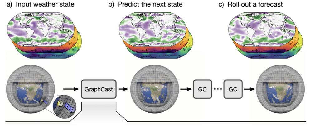
To capture both global and local weather patterns, GraphCast represents the Earth’s atmosphere using graph meshes at multiple resolutions:
- Coarse meshes provide a global context for large-scale weather patterns.
- Fine meshes capture localized phenomena such as storms or temperature gradients.
This hierarchical graph representation allows GraphCast to effectively balance computational efficiency with high-resolution predictive accuracy, making it one of the most advanced GNN-based weather forecasting systems to date.
Conclusions
Graph Neural Networks (GNNs) extend traditional neural networks to graph-structured data, effectively combining node features with the underlying graph topology.
- GNNs operate through message passing, where each node updates its representation by aggregating information from its neighbors.
- Different GNN variants—such as GCN, GAT, GATv2, and others—introduce alternative mechanisms for aggregation and weighting, enabling more flexible and expressive modeling of complex graphs.
- GNNs have proven effective across a variety of tasks:
- Node classification – labeling individual nodes based on features and neighborhood context
- Link prediction – predicting the existence or type of edges between nodes
- Graph classification – assigning labels to entire graphs
- Applications span social networks, biological networks, recommendation systems, and many more domains.
- Despite their successes, challenges remain, including scalability to very large graphs, over-smoothing of node representations, interpretability of learned embeddings, and handling of dynamic or evolving graphs.
Key Takeaways
| Topic | Key Point |
|---|---|
| From grids to graphs | CNNs assume regular Euclidean grids; GNNs generalize to irregular, non-Euclidean structures |
| Message passing | Core GNN mechanism: each node aggregates neighbor features, then updates its own embedding |
| GCN layer | Uses symmetric normalization of the adjacency matrix with self-loops for stable propagation |
| Adjacency matrix | Encodes graph structure as a fixed prior; enforces locality and reduces overfitting |
| Receptive field | Stacking GNN layers lets each node capture information from its -hop neighborhood |
| Node classification | Predict labels per node; can be transductive (same graph) or inductive (new graphs) |
| Link prediction | Predict edges between node pairs using learned embeddings + decoder |
| Graph classification | Global pooling aggregates all node embeddings into a single graph-level representation |
| GAT | Learns attention coefficients over neighbors instead of using fixed adjacency weights |
| GAT multi-head | Runs independent attention heads in parallel; concatenates outputs for richer representations |
| GraphCast | State-of-the-art weather forecasting using GNNs on multi-resolution spherical meshes |